16Sequence Stratigraphy

Across a seismic section of a continental margin, reflections lap onto older ones, then build out toward the basin, then step back toward the land, and the pattern repeats itself higher up. Each package records a contest between two rates: the rate at which room for sediment is made, by subsidence and by the rise of the sea, and the rate at which rivers fill it. Sequence stratigraphy reads the contest from the geometry of the layers, and cyclostratigraphy reads its clock from their thickness.

You already know

Accommodation, eustasy, relative sea level, subsidence and the sedimentary basin are in the Year 1 volume, in its chapter on diagenesis and sedimentary basins. Marine transgression and regression and the first-order sea-level cycle are in the Year 2 volume, in its chapter on the Phanerozoic Earth; the Milankovitch parameters and climatic precession in its chapter on orbital forcing and the ice ages; the age model in its chapter on climate archives and proxies. Onlap, downlap, toplap, erosional truncation and seismic stratigraphy are in Chapter 2. Fourier series and the Fourier transform are in the mathematics books.

16.1 Accommodation, supply and the shoreline

At any point of a basin the relative sea level rises at the rate $A = \dot E + \sigma$, the eustatic rate plus the subsidence rate (a fall when $A < 0$). Relative sea level at a place is set by the global sea level and by everything that moves the land beneath it: thermal subsidence, the load of the sediment and the flexure it causes, the rebound of the crust after an ice sheet melts, and the slow push of the mantle beneath the plate. Rising relative sea level makes accommodation; sediment fills it. Whether the shoreline moves seaward or landward depends on both, and not on the sea level alone.

Definition 16.1 (Normal and forced regression)

A normal regression is a seaward move of the shoreline while the relative sea level rises: supply outpaces the accommodation made at the shoreline. A forced regression is a seaward move driven by a fall of relative sea level: the shoreline is pushed basinward whatever the supply, and the land left behind is exposed and eroded.

Definition 16.2 (Shoreline trajectory)

The shoreline trajectory is the path of the shoreline through time, drawn in a dip section in the frame of the sediment, so that it shows both the horizontal move of the shoreline and its rise or fall relative to the layers below.

A simple profile makes the contest exact. Behind the shoreline a flat topset of width $W$ lies at sea level; in front of it a foreset of slope $\tan\theta$ runs down to the basin floor, a height $D$ below. The sediment supply $Q$ is a volume per unit time per metre of coastline (an area per unit time in the section).

Proposition 16.3 (Shoreline trajectory)

If relative sea level rises ($A \ge 0$) and the topset aggrades uniformly, the shoreline moves at

$$\frac{\mathrm dx_s}{\mathrm dt} = \frac{Q - AW}{D};$$

it progrades while $Q > AW$ and retreats when $AW > Q$. If relative sea level falls ($A < 0$), the topset receives nothing and

$$\frac{\mathrm dx_s}{\mathrm dt} = \frac{Q}{D} + \frac{|A|}{\tan\theta}.$$

In both cases the trajectory climbs or descends at the angle whose tangent is $A/(\mathrm dx_s/\mathrm dt)$.

A normal regression therefore needs a supply larger than the accommodation made on the topset, and its trajectory climbs; a forced regression happens whatever the supply, and its trajectory descends. The ratio of the two rates, often written $A/S$, sorts the patterns: progradation when $A/S < 1$ on the topset, aggradation near 1, retrogradation above. The same sea-level curve can therefore give a regression on a margin rich in sediment and a transgression on a starved one.

16.2 Stratal geometry: sequences and systems tracts

The reflection terminations of Chapter 2 are the vocabulary of the method: onlap and downlap mark the base of a package, toplap and erosional truncation its top. Read in a dip section, they divide a margin into packages bounded by surfaces of non-deposition or erosion, each recording one cycle of relative sea level.

Definition 16.4 (Depositional sequence and sequence boundary)

A depositional sequence is a succession of genetically related strata, without major break inside, bounded at its base and top by unconformities or by the conformities that continue them into the basin. Its bounding surface is the sequence boundary: an unconformity cut by exposure and erosion on the shelf during a fall of relative sea level, passing basinward into a correlative conformity.

Definition 16.5 (Systems tract)

A systems tract is the set of depositional systems (river, coast, shelf, slope) that were active together during one part of a relative sea-level cycle, recognised by its position in the sequence, its bounding surfaces and its stacking pattern. Four are distinguished:

• the falling-stage systems tract, built by forced regression while relative sea level falls: downstepping foresets detached from the old shelf;
• the lowstand systems tract, built by normal regression once relative sea level starts to rise again, at the lowest shoreline position: a wedge that aggrades and progrades;
• the transgressive systems tract, built while the shoreline retreats landward: backstepping units onlapping the old shelf;
• the highstand systems tract, built by normal regression late in the rise, when supply again outpaces accommodation: foresets that prograde and downlap onto the deposits below.

Definition 16.6 (Transgressive and maximum flooding surfaces)

The transgressive surface is the first significant flooding surface above the lowstand deposits: it marks the turn of the shoreline from regression to transgression. The maximum flooding surface marks the most landward position of the shoreline, the turn from transgression to highstand regression; the highstand foresets downlap onto it.

Definition 16.7 (Condensed section and incised valley)

A condensed section is a thin interval deposited very slowly far from the shoreline while the sea floods the shelf and the sediment is trapped near the coast: a few centimetres or decimetres of clay, fossils, glauconite or phosphate that may record a long time. An incised valley is a river valley cut into the exposed shelf while relative sea level falls, and filled during the following lowstand and transgression.

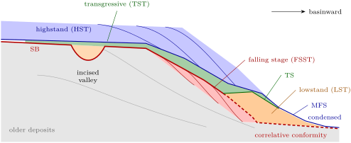
Where exactly the sequence boundary runs in the basin is a convention, and authors differ: some draw it at the base of the falling-stage deposits, where the fall begins, others at their top, where it ends, as in the figure above. On the shelf there is no ambiguity: the boundary is the surface of exposure and erosion, and the deposits above it are younger than the fall.

Read from the bottom up at one place on the outer shelf, a sequence records the cycle: highstand foresets, a surface of exposure, perhaps a valley fill, the transgressive surface, backstepping beds, a condensed interval at the maximum flooding surface, then highstand foresets again. The hierarchy of cycles is set by their causes: the opening and closing of oceans for the first-order cycle, changes in ice volume and in the speed of sea-floor spreading for the shorter ones, and local tectonics and supply for all of them.

16.3 Parasequences and stacking patterns

Inside a systems tract the smallest packages a geologist maps on a cliff or a well log are shallowing-upward units a few metres to a few tens of metres thick, capped by a surface where deeper water suddenly returns.

Definition 16.8 (Parasequence and flooding surface)

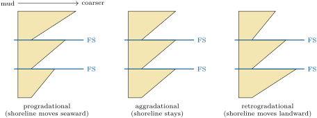
A parasequence is a relatively conformable succession of genetically related beds bounded by flooding surfaces, in which the water shallows upward: on a wave-dominated coast, offshore mud passes up into lower and upper shoreface sand and beach. A flooding surface is a surface across which deeper-water facies abruptly overlie shallower ones, with evidence of a sudden deepening.

A single parasequence coarsens upward, and its gamma-ray log, low in sand and high in clay, makes a funnel shape that narrows upward. How the parasequences of a tract stack upon one another tells the trend of the shoreline: each one built farther seaward than the last (progradational), above the last (aggradational), or landward of it (retrogradational). A log through the stack shows the trend directly: each parasequence ending in coarser, shallower facies than the one below, the same, or finer and deeper. Highstand and lowstand tracts stack progradationally or aggradationally, transgressive tracts retrogradationally. The next chapter reads such logs facies by facies.

In the field — Parasequences in a desert cliff

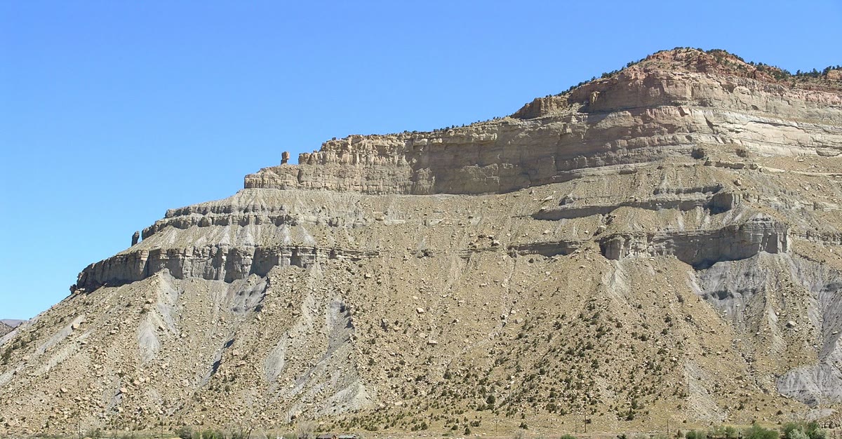
The Book Cliffs of eastern Utah expose Upper Cretaceous shoreline deposits for tens of kilometres. In the Kenilworth Member, followed along the cliffs from Price to Hatch Mesa, geologists mapped coastal-plain, shoreface, inner-shelf and incised-valley deposits, and nine coarsening-upward, wave- to storm-dominated parasequences 7 to $32\,\mathrm{m}$ thick. Basinward each splits into up to four smaller coarsening-upward bedsets, 2 to $18\,\mathrm{m}$ thick; some shoreface sands rest on a sharp base, which the study reads as deposits of a lowstand.

16.4 A forward model of a shelf

The rules of the previous sections can be run as a model. The Varden basin is an invented shelf: a ramp sloping basinward at $1.5\,\mathrm{m}/\mathrm{km}$, subsiding at $\sigma = 0.02 + x/1200$ $\mathrm{m}/\mathrm{kyr}$ at a distance $x$ (km) from the hinge, under a sea level $E = -30\cos(2\pi t/400)$ (m, $t$ in kyr), fed by a river supplying $Q = 6000\,\mathrm{m}^{3}/\mathrm{kyr}$ per metre of coast. At every step of half a thousand years the basin subsides; the sediment then fills a flat topset up to sea level, wherever the old surface is under water, and a foreset of slope 0.012 in front of it, the shoreline being placed so that the volume added equals the supply; exposed land receives nothing and, for simplicity, is not eroded. The model starts at a lowstand, after a first wedge built at constant sea level.

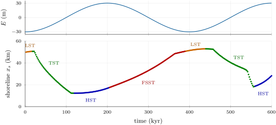
The figure above follows the shoreline through time, and the one below shows the deposits it left. The tracts appear with no rule written into the model beyond filling and subsidence. The lowstand wedge at the start sits far out; the rising sea drives the shoreline $38\,\mathrm{km}$ landward in the first transgression, and the highstand foresets build out again as the rise slows. Then the fall begins: the shoreline is pushed basinward by $33\,\mathrm{km}$ in $187\,\mathrm{kyr}$, leaving thin downstepping foresets and an exposed shelf behind, the falling-stage tract. A new lowstand wedge, a second transgression and a new highstand follow. The speed of the forced regression in the model matches the formula of the proposition to within a few per cent; under a rising sea the model’s topset does not aggrade uniformly, since subsidence grows basinward, and the formula is only a guide.

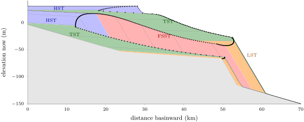
The relative sea level begins to fall at the shoreline a few thousand years after the eustatic highstand, because the subsidence must first be overtaken, and it ends a few thousand years before the eustatic lowstand. The fall at the shoreline thus lasts less than half the eustatic cycle, and the more so the faster the basin subsides.

Models of this kind are the honest test of an interpretation, and also show its limits. The same section can be built by different histories: a faster fall with less supply, or a slower one with more, or a change of subsidence rather than of sea level, since the geometry only records the relative sea level and the supply. Global charts of sea-level cycles built from margins in the 1970s and 1980s fixed the timing of many falls that drilling has since largely confirmed for parts of the Late Cretaceous to Miocene, but their amplitudes, such as a fall of $160\,\mathrm{m}$ in the middle Oligocene, are too high by a factor of 2 to 3. Eustatic amplitudes are now taken from oxygen isotopes and from backstripped wells, and a margin’s sequences are read first as a local record.

16.5 Cyclostratigraphy

Many successions repeat themselves at regular thickness intervals: couplets of marl and limestone, bundles of five couplets, larger sets of bundles. If the repetition is paced by the Milankovitch parameters, the thickness of the cycles turns into time.

Definition 16.9 (Cyclostratigraphy and astronomical tuning)

Cyclostratigraphy identifies and measures regular cycles in sedimentary successions and interprets them as records of periodic forcing, mainly the variations of the Earth’s orbit and axis. Astronomical tuning assigns ages to a succession by matching its cycles, one by one, to a computed astronomical series (eccentricity, obliquity, precession or insolation), which turns the cycles into an age model.

The computed periods come from the solution of the Solar System’s motion. The eccentricity of the Earth’s orbit has a main term of $405\,\mathrm{kyr}$, and four terms near $100\,\mathrm{kyr}$ (95, 99, 124 and $131\,\mathrm{kyr}$); the obliquity a main term of $41.0\,\mathrm{kyr}$ with smaller ones at 39.6 and $53.7\,\mathrm{kyr}$. Climatic precession combines the precession of the axis with the motion of the perihelion, at frequencies $p_0 + g_i$, where $p_0 = 50.47''$ per year and the $g_i$ are frequencies of the planetary orbits; its main periods are 23.7, 22.4, 19.1 and $19.0\,\mathrm{kyr}$. The $405\,\mathrm{kyr}$ term is the steadiest, and serves as a metronome for older successions.

Definition 16.10 (Periodogram)

The periodogram of a series $y_0, \dots, y_{N-1}$ sampled at a step $\Delta$ (in time or depth), after removal of its mean and trend and multiplication by a taper $w_k$, is

$$P(f_j) = \Bigl|\sum_{k=0}^{N-1} w_k y_k\, e^{-2\pi i f_j k\Delta}\Bigr|^2, \qquad f_j = \frac{j}{N\Delta},\ j = 1, \dots, \frac N2:$$

the power of the series at each frequency $f_j$, the square of the modulus of its discrete Fourier transform.

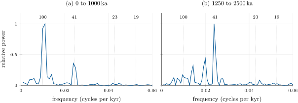
Two numbers bound what a periodogram can see. Its frequency step, $1/(N\Delta)$, the inverse of the record’s length, is the resolution: two periods whose frequencies differ by less cannot be separated. Its highest frequency, the Nyquist frequency $1/(2\Delta)$, is reached with two samples per cycle; a shorter cycle is not lost but folded back to a false longer one. The taper, here a Hann window, smooths the ends of the series so that a strong peak does not leak power across the whole spectrum.

The periodograms above are the worked case. In the last million years the strongest peak falls in the $100\,\mathrm{kyr}$ band (at $91\,\mathrm{kyr}$ on the frequency grid of a $1000\,\mathrm{kyr}$ record, whose neighbours are 100 and $83\,\mathrm{kyr}$), the obliquity has a third of its power and the precession a few per cent; between 2.5 and $1.25\,\mathrm{Ma}$ the obliquity carries the record and the $100\,\mathrm{kyr}$ band has a sixth of its power. One caution is built into the data: the LR04 time scale was itself obtained by tuning the stack to a simple ice model driven by summer insolation at $65{}^{\circ}$ N, constrained by stacked sedimentation rates to prevent overtuning, so finding orbital periods in it is partly circular. The test that is not circular is the one done in depth, before any tuning: if the ratios of the thicknesses of the cycles match the ratios of the orbital periods, the forcing is shown, and the thicknesses give the sedimentation rate.

Method 16.11 (Sedimentation rate from cycle thickness)

1. compute the periodogram of the series in depth, with its resolution $1/L$ for a section of length $L$ and its Nyquist limit $1/(2\Delta z)$;
2. list the wavelengths of the significant peaks, $\lambda = 1/f$;
3. compare their ratios with those of the orbital periods (405 : 100 : 41 : 23, or 21 for an average precession); a match of three peaks is a strong argument, one peak alone none;
4. divide each wavelength by its period: the quotients, which should agree, give the sedimentation rate.

A sedimentation rate obtained this way is an average over the cycle and assumes a steady rate: a change of rate within the section stretches the peaks, and a hiatus removes cycles silently. Long successions are therefore tuned cycle by cycle against the computed series, the $405\,\mathrm{kyr}$ cycle first, and checked against radiometric ages where volcanic beds allow.

16.6 Exercises

Exercise 16.1 ★

At a point of a shelf the eustatic sea level rises at $0.5\,\mathrm{m}/\mathrm{kyr}$ and the basin subsides at $0.1\,\mathrm{m}/\mathrm{kyr}$. Compute the rate of relative sea-level rise and the accommodation made in $20\,\mathrm{kyr}$. What is the relative rate if the sea falls at $0.3\,\mathrm{m}/\mathrm{kyr}$ instead?

Solution

Solution of Exercise 16.1.

$A = 0.5 + 0.1 = 0.6\,\mathrm{m}/\mathrm{kyr}$; in $20\,\mathrm{kyr}$, $12\,\mathrm{m}$ of accommodation. With the sea falling, $A = -0.3 + 0.1 = -0.2\,\mathrm{m}/\mathrm{kyr}$: a relative fall, slowed by the subsidence.

Exercise 16.2 ★

For each case, name the systems tract being built: (a) relative sea level falls, the shoreline moves seaward; (b) relative sea level rises, the shoreline moves landward; (c) relative sea level rises slowly late in a cycle, the shoreline moves seaward and the foresets downlap onto a surface of maximum flooding; (d) relative sea level has just begun to rise after a fall, and the shoreline still moves seaward.

Solution

Solution of Exercise 16.2.

(a) Falling-stage tract (forced regression). (b) Transgressive tract. (c) Highstand tract. (d) Lowstand tract (normal regression after the fall).

Exercise 16.3 ★

A well log shows three parasequences, each coarsening upward. The tops of the three, from the lowest, are fine sand, medium sand and coarse sand with beach lamination. Name the stacking pattern, the move of the shoreline and the systems tracts it may belong to. What would the opposite order mean?

Solution

Solution of Exercise 16.3.

Each parasequence ends shallower than the one below: a progradational stack, the shoreline moving seaward, as in a highstand or a lowstand tract. The opposite order, each ending finer and deeper, is retrogradational: a transgressive tract.

Exercise 16.4 ★

A cliff shows couplets of marl and limestone grouped in bundles of five; a bundle is $1.6\,\mathrm{m}$ thick. Interpret the couplets and the bundles with the orbital periods, and compute the sedimentation rate from the bundles.

Solution

Solution of Exercise 16.4.

Five couplets to a bundle is the ratio of the short eccentricity (about $100\,\mathrm{kyr}$) to the precession (about $20\,\mathrm{kyr}$): each couplet is a precession cycle, each bundle an eccentricity cycle. The rate is $1.6/100 = 1.6\,\mathrm{cm}/\mathrm{kyr}$, and a couplet of $0.32\,\mathrm{m}$ lasts about $20\,\mathrm{kyr}$, consistent.

Exercise 16.5 ★★

A shelf has a topset $20\,\mathrm{km}$ wide, a foreset $50\,\mathrm{m}$ high, and a supply of $4000\,\mathrm{m}^{3}/\mathrm{kyr}$ per metre of coast; relative sea level rises at $0.15\,\mathrm{m}/\mathrm{kyr}$. Compute the speed of the shoreline. At what rate of rise would it stand still?

Solution

Solution of Exercise 16.5.

$\mathrm dx_s/\mathrm dt = (4000 - 0.15\times20\,000)/50 = 20\,\mathrm{m}/\mathrm{kyr}$, seaward. The shoreline stands still when $AW = Q$: $A = 4000/20\,000 = 0.2\,\mathrm{m}/\mathrm{kyr}$.

Exercise 16.6 ★★

The same shelf now sees its relative sea level fall at $0.2\,\mathrm{m}/\mathrm{kyr}$; the foreset slope is 0.01. Compute the speed of the forced regression and the share of it that is due to the fall alone.

Solution

Solution of Exercise 16.6.

$\mathrm dx_s/\mathrm dt = 4000/50 + 0.2/0.01 = 80 + 20 = 100\,\mathrm{m}/\mathrm{kyr}$; the fall alone accounts for $20\,\mathrm{m}/\mathrm{kyr}$, a fifth.

Exercise 16.7 ★★

Relative sea level rises at $0.4\,\mathrm{m}/\mathrm{kyr}$ over a topset $25\,\mathrm{km}$ wide. Below what supply does the shoreline retreat? With a supply of $6000\,\mathrm{m}^{3}/\mathrm{kyr}$ per metre and a shoreface only $10\,\mathrm{m}$ high, how fast does it retreat?

Solution

Solution of Exercise 16.7.

It retreats when $Q < AW = 0.4\times25\,000 = 10\,000\,\mathrm{m}^{3}/\mathrm{kyr}$ per metre. With $Q = 6000$: $(6000 - 10\,000)/10 = -400\,\mathrm{m}/\mathrm{kyr}$, a retreat of $0.4\,\mathrm{km}$ every thousand years: a low shoreface makes a fast transgression.

Exercise 16.8 ★★

The eccentricity terms of 94.9 and $123.9\,\mathrm{kyr}$, and those of 94.9 and $98.9\,\mathrm{kyr}$: how long a record is needed to separate each pair in a periodogram? Can a $600\,\mathrm{kyr}$ record do it?

Solution

Solution of Exercise 16.8.

$1/94.9 - 1/123.9 = 0.002\,47\text{ cycles}/\mathrm{kyr}$: a record longer than $1/0.00247 = 406\,\mathrm{kyr}$ separates them, and $600\,\mathrm{kyr}$ (resolution 0.00167) is enough. $1/94.9 - 1/98.9 = 0.00042$: it needs about $2400\,\mathrm{kyr}$, four times longer than the record.

Exercise 16.9 ★★

In a core, 20 obliquity cycles ($40.98\,\mathrm{kyr}$ each) occupy $16.4\,\mathrm{m}$. Compute the sedimentation rate, and the time between two ash beds $3.1\,\mathrm{m}$ apart in the same interval.

Solution

Solution of Exercise 16.9.

$16.4/(20\times40.98) = 0.0200\,\mathrm{m}/\mathrm{kyr}$, $2.0\,\mathrm{cm}/\mathrm{kyr}$; the ash beds are $3.1/0.020 = 155\,\mathrm{kyr}$ apart.

Exercise 16.10 ★★★

Compute the angle of the shoreline trajectory (a) in a forced regression at $200\,\mathrm{m}/\mathrm{kyr}$ with relative sea level falling at $0.4\,\mathrm{m}/\mathrm{kyr}$, (b) in a normal regression at $50\,\mathrm{m}/\mathrm{kyr}$ with relative sea level rising at $0.2\,\mathrm{m}/\mathrm{kyr}$. Why is an angle of a fraction of a degree easy to see on a seismic section and hard to see on a cliff?

Solution

Solution of Exercise 16.10.

(a) $\tan\alpha = -0.4/200 = -0.002$: descending at $0.11{}^{\circ}$. (b) $0.2/50 = 0.004$: climbing at $0.23{}^{\circ}$. A seismic section spans tens of kilometres at a vertical exaggeration of tens to hundreds, so the angle shows; a cliff a few hundred metres long shows a rise of a metre or less, lost in the variation of the beds.

Exercise 16.11 ★★★

The precession constant is $p_0 = 50.467718''$ per year and four planetary frequencies are $g_5 = 4.257564$, $g_2 = 7.456665$, $g_4 = 17.910194$ and $g_3 = 17.366595''$ per year. Compute the periods of climatic precession $1\,296\,000''/(p_0 + g_i)$. Check that $g_2 - g_5$ and $g_4 - g_5$ give the 405 and $95\,\mathrm{kyr}$ eccentricity terms.

Solution

Solution of Exercise 16.11.

$1\,296\,000/54.725282 = 23.68\,\mathrm{kyr}$ ($g_5$); $/57.924383 = 22.37\,\mathrm{kyr}$ ($g_2$); $/68.377912 = 18.95\,\mathrm{kyr}$ ($g_4$); $/67.834313 = 19.11\,\mathrm{kyr}$ ($g_3$). $g_2 - g_5 = 3.199101''$ per year, $405.1\,\mathrm{kyr}$; $g_4 - g_5 = 13.65263''$, $94.9\,\mathrm{kyr}$.

Exercise 16.12 ★★★

Two basins record the same relative sea-level rise of $0.3\,\mathrm{m}/\mathrm{kyr}$ for $100\,\mathrm{kyr}$. In the first, eustasy rises at $0.25\,\mathrm{m}/\mathrm{kyr}$ and the basin subsides at $0.05\,\mathrm{m}/\mathrm{kyr}$; in the second, eustasy rises at $0.1\,\mathrm{m}/\mathrm{kyr}$ and the basin subsides at $0.2\,\mathrm{m}/\mathrm{kyr}$. Show that the two sections can be identical. What extra observation separates the two histories?

Solution

Solution of Exercise 16.12.

Both make $0.3\times100 = 30\,\mathrm{m}$ of accommodation at the same rate; with the same supply the geometry is the same, since sediment responds only to the relative sea level. A eustatic change is the same everywhere: the same sequence, of the same age, on other margins points to the first history. A subsidence history built from the basin’s thermal and load history (backstripping), or an independent eustatic record such as oxygen isotopes, separates them too.

16.7 Problem: Sea Levels of the Varden Basin

Problem 16.1

Weekend problem — accommodation, the shoreline trajectory and the systems tracts of the Varden shelf model, and the clock of a core

The Varden shelf of the chapter subsides at $\sigma = 0.02 + x/1200$ ($\mathrm{m}/\mathrm{kyr}$, $x$ in km), under a sea level $E = -30\cos(2\pi t/400)$ (m, $t$ in kyr), with a supply of $6000\,\mathrm{m}^{3}/\mathrm{kyr}$ per metre of coast and a foreset slope of 0.012. The model gives, every $50\,\mathrm{kyr}$, the sea level $E$, the shoreline position $x_s$, the rate of relative sea-level rise at the shoreline $A$ and the height $D$ of the foreset:

$t$	$E$	$x_s$	$A$	$D$	$t$	$E$	$x_s$	$A$	$D$
(kyr)	(m)	(km)	(m/kyr)	(m)	(kyr)	(m)	(km)	(m/kyr)	(m)
50	$-21.2$	33.5	0.381	–	350	$-21.2$	44.6	$-0.276$	25.3
100	0.0	15.7	0.504	–	400	$-30.0$	51.3	0.063	81.6
150	21.2	12.8	0.364	21.1	450	$-21.2$	52.7	0.397	99.2
200	30.0	16.8	0.034	41.1	500	0.0	40.4	0.525	–
250	21.2	24.0	$-0.293$	45.4	550	21.2	22.9	0.372	–
300	0.0	32.9	$-0.424$	35.7	600	30.0	28.2	0.043	13.4

(A dash marks a shoreline retreating over a flat coastal plain, where no foreset is built.)

Part I — Accommodation.

1. Compute the largest eustatic rate and when it occurs.
2. Compute the subsidence rate at the hinge, at 20 and $50\,\mathrm{km}$, and at the edge of the model, $120\,\mathrm{km}$.
3. The shoreline stands near $17.5\,\mathrm{km}$ at the highstand. When does relative sea level begin to fall there?
4. The shoreline reaches about $50\,\mathrm{km}$ near the lowstand. When does relative sea level stop falling there?
5. How long does the relative fall at the shoreline last, compared with the $200\,\mathrm{kyr}$ of the eustatic fall? Why is it shorter?
6. How much accommodation does subsidence alone make in one cycle at $30\,\mathrm{km}$? Compare it with the eustatic range.

Part II — The shoreline.

7. Read the table: between which times does the shoreline move seaward, and between which landward?
8. A highstand topset $15\,\mathrm{km}$ wide aggrades at $0.30\,\mathrm{m}/\mathrm{kyr}$ in front of a foreset $40\,\mathrm{m}$ high. Compute the speed of the shoreline with the proposition of the chapter.
9. On that topset, at what rate of rise would the shoreline stop?
10. At $300\,\mathrm{kyr}$, compute the speed of the forced regression from the table. The model gives $204\,\mathrm{m}/\mathrm{kyr}$: compare.
11. Which of the two terms dominates, the supply or the fall?
12. The trajectory descends from $16.3\,\mathrm{m}$ at $17.4\,\mathrm{km}$ ($204.5\,\mathrm{kyr}$) to $-42.7\,\mathrm{m}$ at $50.7\,\mathrm{km}$ ($391.5\,\mathrm{kyr}$), in present elevations. Compute its mean gradient. From the subsidence each point has undergone since, show why the descent nearly equals the eustatic fall of $59.7\,\mathrm{m}$.

Part III — The systems tracts.

13. From the table, assign a systems tract to each time from 150 to $600\,\mathrm{kyr}$.
14. The model places the onset of the falling stage at $204.5\,\mathrm{kyr}$ and its end at $391.5\,\mathrm{kyr}$: check them against questions 3 and 4.
15. Where does the sequence boundary form in this model, on the shelf and in the basin? The model does not erode: what would a real shelf show?
16. The second transgression ends at $559\,\mathrm{kyr}$ with the shoreline at $18.5\,\mathrm{km}$. Compute its mean speed from its start at $52.8\,\mathrm{km}$ at $439.5\,\mathrm{kyr}$. Which surface forms at its end?
17. Why is the transgressive tract thin on the shelf, and where would a condensed section form?

Part IV — A core from the basin. A core $30\,\mathrm{m}$ long, sampled every centimetre, shows a regular alternation; its periodogram in depth has peaks at wavelengths of 7.5, 2.0 and $0.81\,\mathrm{m}$, the largest at $2.0\,\mathrm{m}$.

18. Compute the frequency resolution and the Nyquist frequency of the periodogram.
19. Compute the ratios of the three wavelengths to the largest peak, and compare them with the orbital periods.
20. Assign periods to the peaks and compute the sedimentation rate from each. Why does the longest disagree slightly?
21. How long a time does the core cover?
22. At what wavelength should the precession of $23.7\,\mathrm{kyr}$ appear? Could a core sampled every $25\,\mathrm{cm}$ see it, and where would it fall?
23. Why is a match of three peaks a stronger argument than one?
24. State the maximum basinward shift of the shoreline in the model, from the start of the fall to the end of the lowstand regression.

Solution

Solution of Problem 16.1.

1. $\dot E = 30\times2\pi/400\times\sin(2\pi t/400)$: at most $0.471\,\mathrm{m}/\mathrm{kyr}$, rising at $100\,\mathrm{kyr}$ and $500\,\mathrm{kyr}$, falling at $300\,\mathrm{kyr}$.

2. $0.020\,\mathrm{m}/\mathrm{kyr}$ at the hinge, 0.037 at $20\,\mathrm{km}$, 0.062 at $50\,\mathrm{km}$, $0.120\,\mathrm{m}/\mathrm{kyr}$ at $120\,\mathrm{km}$.

3. $A < 0$ when $\sin(2\pi t/400) < -0.0346/0.471 = -0.0734$: $t = 200 + (400/2\pi)\arcsin0.0734 = 204.7\,\mathrm{kyr}$.

4. With $\sigma = 0.0617$: $t = 400 - 63.66\arcsin0.131 = 391.6\,\mathrm{kyr}$.

5. About $187\,\mathrm{kyr}$ against 200: the eustatic fall must first overtake the subsidence, and stops beating it before the lowstand.

6. $0.045\times400 = 18\,\mathrm{m}$, against a eustatic range of $60\,\mathrm{m}$: a third.

7. Landward from 50 to about $120\,\mathrm{kyr}$, seaward to about $440\,\mathrm{kyr}$, landward to about $560\,\mathrm{kyr}$, seaward again to $600\,\mathrm{kyr}$ (the model’s turning points are 118.5, 439.5 and $559\,\mathrm{kyr}$; a table every $50\,\mathrm{kyr}$ only brackets them).

8. $(6000 - 0.30\times15\,000)/40 = 37.5\,\mathrm{m}/\mathrm{kyr}$, seaward.

9. $6000/15\,000 = 0.40\,\mathrm{m}/\mathrm{kyr}$.

10. $6000/35.7 + 0.424/0.012 = 168.1 + 35.3 = 203\,\mathrm{m}/\mathrm{kyr}$, within $0.5\,\%$ of the model.

11. The supply: $83\,\%$ of the speed.

12. $(-42.7 - 16.3)/(50.7 - 17.4) = -1.77\,\mathrm{m}/\mathrm{km}$, $0.10{}^{\circ}$. Since its time, the first point has subsided $0.0345\times395.5 = 13.6\,\mathrm{m}$, the second $0.0623\times208.5 = 13.0\,\mathrm{m}$: nearly the same, so in present elevations the descent, $59.0\,\mathrm{m}$, differs from the eustatic fall only by $0.6\,\mathrm{m}$. The relative fall at the shoreline at the time, eustasy minus the subsidence during the fall, was smaller.

13. 150 and 200: highstand; 250, 300, 350: falling stage; 400: lowstand; 450, 500, 550: transgressive (the shoreline retreats just after 440); 600: highstand.

14. 204.7 and $391.6\,\mathrm{kyr}$ against 204.5 and 391.5: the same, within the model’s step of $0.5\,\mathrm{kyr}$.

15. On the shelf, the surface exposed during the fall: the top of the highstand deposits from the hinge to $17\,\mathrm{km}$, continued over the downstepping falling-stage foresets; in the basin, the correlative conformity at the base or top of the falling-stage tract, by convention. A real shelf would be cut by rivers into incised valleys, weathered into soils, and partly eroded.

16. $(18.5 - 52.8)/(559 - 439.5) = -0.29\,\mathrm{km}/\mathrm{kyr}$; the maximum flooding surface forms at its end.

17. The shoreline sweeps quickly over a nearly flat coastal plain: the supply is trapped near it, spread over a wide area, and each place receives little. Basinward of the toe, beyond about $55\,\mathrm{km}$, the sea floor is starved: a condensed section forms there.

18. Resolution $1/30 = 0.033\text{ cycles}/\mathrm{m}$; Nyquist $1/(2\times 0.01) = 50\text{ cycles}/\mathrm{m}$.

19. $7.5/2.0 = 3.75$, 1 and $0.81/2.0 = 0.405$; the orbital ratios are $405/100 = 4.05$ and $41/100 = 0.41$.

20. $2.0\,\mathrm{m}$ for $100\,\mathrm{kyr}$: $2.0\,\mathrm{cm}/\mathrm{kyr}$; $0.81/41 = 1.98\,\mathrm{cm}/\mathrm{kyr}$; $7.5/405 = 1.85\,\mathrm{cm}/\mathrm{kyr}$. The wavelengths the periodogram can show near $8\,\mathrm{m}$ are 10, 7.5 and $6\,\mathrm{m}$: the true $8.1\,\mathrm{m}$ falls between two of them.

21. $30/0.020 = 1500\,\mathrm{kyr}$.

22. $23.7\times0.020 = 0.474\,\mathrm{m}$. Sampled every $25\,\mathrm{cm}$, the Nyquist frequency is 2 cycles per metre, a wavelength of $0.5\,\mathrm{m}$: the precession, at 2.11 cycles per metre, is beyond it and folds back to $4 - 2.11 = 1.89$, a false wavelength of $0.53\,\mathrm{m}$.

23. A single peak fits some period at some rate whatever its origin; three peaks whose ratios match the orbital ratios are independent of the rate, which must then come out the same from each.

24. The shoreline moves from $17.37\,\mathrm{km}$ at the start of the fall to $52.84\,\mathrm{km}$ at the end of the lowstand regression: a maximum basinward shift of $35.5\,\mathrm{km}$.