University Earth and Space Sciences — Year 3 · 本科三年级
5Thermal Models of the Lithosphere
Sail away from a mid-ocean ridge and the sea floor deepens: about 2.5km at the axis, more than 5km beneath the oldest ocean floor. Nothing has been added to the plate or taken away from it; it has only cooled, contracted and sunk. The ocean floor is a thermometer of the plate beneath it, and a heat-flow probe pushed into its sediment reads the same cooling from above. This chapter solves the cooling of a plate in two ways, as a half-space and as a plate of finite thickness, compares both with the depth of the real ocean floor and its heat flow, and then turns to the continents, whose heat comes partly from their own crust.
You already know
The diffusion equation for heat, ∂T/∂t=κ∇2T, with the thermal conductivity k and the thermal diffusivity κ=k/(ρc), is the physics books’; Fourier series and the error function erfx=(2/π)∫0xe−u2du are in the mathematics books’ university volumes. The heat flow, the radiogenic heat production, the geotherm, the conductive time scale L2/κ, the thermal boundary layer and the thermal lithosphere were defined in the Year 1 volume, in its chapter on the Earth’s heat budget; isostasy in its chapter on isostasy and gravity anomalies; the depth–age law d=dr+Ct was proved in its chapter on rifts, ridges and passive margins, admitting the temperature profile that this chapter derives. The stretching model of basins, post-rift subsidence and the thermal time constant are in the Year 2 volume, in its chapter on sedimentary basins.
5.1 Conduction, advection and their ratio
Heat in the lithosphere moves in two ways: it diffuses down the temperature gradient, and it is carried by moving rock, the plate leaving a ridge, an eroded mountain rising, a magma ascending. Which one wins depends on a single number.
Definition 5.1(Thermal Péclet number)
For rock moving at the speed u across a length L, the thermal Péclet number is
Pe=κuL,
the ratio of the conductive time L2/κ to the advective time L/u. Advection dominates where Pe≫1, conduction where Pe≪1.
A plate leaving a ridge at 25mm/yr has, over a distance of 95km, Pe≈94 with κ=0.8×10⁻⁶m2s−1: heat is carried sideways by the plate far faster than it diffuses sideways. Each vertical column of the plate therefore cools as if alone, by vertical conduction to the cold sea floor, its age t standing for the time since it left the axis. That turns a problem in two dimensions into one in depth and time.
5.2 The cooling half-space
Definition 5.2(Half-space cooling model)
The half-space cooling model of the oceanic lithosphere takes each column as a half-space z≥0 of uniform diffusivity, at the uniform temperature Tm of the mantle when it leaves the ridge axis, whose surface is held from then on at the temperature T0 of the sea floor, with no heat production and no bottom.
Proof. Let θ=(T−T0)/(Tm−T0); it solves ∂θ/∂t=κ∂2θ/∂z2 with θ(z,0)=1 for z>0 and θ(0,t)=0 for t>0. The problem has no length scale of its own: if θ(z,t) is a solution, so is θ(λz,λ2t) for every λ>0, with the same initial and boundary values; the solution being unique, θ depends on z and t only through η=z/(2κt). Writing θ=f(η), with ∂η/∂t=−η/(2t) and ∂η/∂z=1/(2κt),
−2tηf′(η)=κ4κtf′′(η),sof′′+2ηf′=0.
Hence f′=Ae−η2 and f=A∫0ηe−u2du+B. The surface condition, at η=0, gives B=0; the initial condition, which holds at every depth as t→0, that is as η→∞, gives Aπ/2=1. So f=erfη. ∎
The temperature at a given depth depends only on z/t: an isotherm sinks as the square root of age, and the cooled layer at 40Myr is twice as thick as at 10Myr. The surface heat flow follows by differentiation.
Proof.∂erf(z/2κt)/∂z=(2/π)e−z2/4κt/(2κt), which at z=0 is 1/πκt. ∎
With the values of the plate model below (k=3.1Wm−1K−1, Tm−T0=1450K, κ=0.8×10⁻⁶m2s−1), Cq=505mWm−2Myr1/2, close to the values of 430 to 510mWm−2Myr1/2 fitted to the global measurements by different studies; a recent compilation prefers 490. Measured heat flow on young oceanic crust, however, grossly underestimates the heat that leaves it: sea water circulating through the cracked crust carries part of the heat away in hot springs, out of reach of the probes. Over old crust the measurements follow 1/t, and estimates of the Earth’s heat loss replace the measurements on crust younger than 66.5Myr with Cq/t.
The Year 1 volume integrated the same profile over depth, through isostasy, to obtain the depth–age law, d=dr+Ct with C=2ρmα(Tm−T0)κ/(π(ρm−ρw)) (figure below). With ρm=3300kgm−3, ρw=1030kgm−3 and α=3.1×10⁻⁵K−1, C=370mMyr−1/2, against the 350mMyr−1/2 fitted to the North Pacific and North Atlantic floors younger than 70Myr.
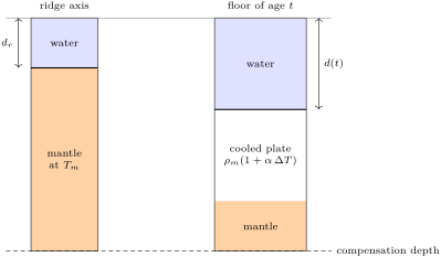
Isostasy of the cooling plate: the column at the ridge and the column of age t have the same mass above the compensation depth. The cooled, denser plate sinks, and water fills the space above it.
5.3 The plate model
Old ocean floor stops deepening: in the North Pacific and North Atlantic the depth departs from t between 60 and 80Myr, and heat flow levels off. The half-space keeps cooling for ever; something must hold the base of the plate warm.
Definition 5.5(Plate cooling model)
The plate cooling model of the oceanic lithosphere takes each column as a layer 0≤z≤L of uniform diffusivity, at the uniform temperature Tm when it leaves the ridge, whose surface is held at T0 and whose base is held at Tm from then on.
Proof. The steady state, reached as t→∞, is the linear profile Tmz/L. The departure u=T−Tmz/L solves the diffusion equation with u=0 at z=0 and z=L, and starts as u(z,0)=Tm(1−z/L). Separating the variables, u=Z(z)Θ(t) gives Z′′/Z=Θ′/(κΘ)=−μ2; the boundary conditions leave Z=sin(nπz/L), μ=nπ/L, and Θ=e−n2π2κt/L2=e−n2t/τ. The initial values fix the coefficients bn of the sine series of Tm(1−z/L) on [0,L]:
bn=L2∫0LTm(1−Lz)sinLnπzdz=nπ2Tm,
by an integration by parts. Summing the modes gives the series. ∎
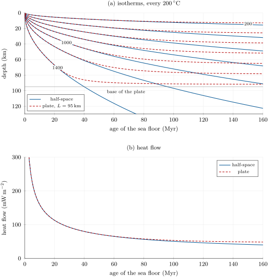
Each mode decays with its own time, τ/n2: the higher harmonics, the fine structure of the initial step, vanish first, and after a time of order τ only the first one is left. The same separation of variables gives the heat flow and, through the isostatic balance of the figure above, the depth.
Proposition 5.7(Depth and heat flow of the plate model)
In the plate cooling model, with the densities and expansion of the depth–age law,
As t→∞, the depth tends to dr+ρmαTmL/(2(ρm−ρw)) and the heat flow to kTm/L, both exponentially, with the time constant τ.
Proof. Differentiating the series at z=0, ∂T/∂z=(Tm/L)[1+2∑e−n2t/τ]. For the depth, the isostatic balance gives (ρm−ρw)(d−dr)=ρmα∫0L(Tm−T)dz. The linear part contributes TmL/2; each mode contributes −(2Tm/nπ)e−n2t/τ∫0Lsin(nπz/L)dz=−(2Tm/nπ)(L/nπ)(1−cosnπ)e−n2t/τ, which is zero for even n and −(4TmL/n2π2)e−n2t/τ for odd n. Factoring TmL/2 gives the bracket. At t=0 it vanishes, since ∑nodd1/n2=π2/8. ∎
The plate model that best fits the global depths and heat flows has a plate 95km thick with a base at 1450∘C, α=3.1×10⁻⁵K−1 and k=3.1Wm−1K−1, thinner and hotter than the earlier 125km and 1350∘C. With κ=0.8×10⁻⁶m2s−1, τ=36.2Myr; the depth levels off at 2500+3104=5604m and the heat flow at 47mWm−2. Young floor cannot tell the two models apart: they differ by less than a metre at 2Myr, by 100m at 44Myr. Seismology gives a similar answer: Pacific Rayleigh waves are best fitted by cooling plates whose asymptotic thickness is 85 to 95km.
The two cooling models with the parameters of the text. (a) Depth of the isotherms from 200∘C (top) to 1400∘C (bottom): those of the half-space go on sinking as t, those of the plate stop as the profile becomes linear. (b) Surface heat flow: the plate model levels off at 47mWm−2, the half-space falls as 1/t.
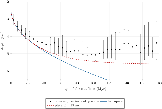
The real ocean floor can be put on the same graph (figure below). Every cell of one degree of latitude and longitude whose age is known is placed at its age and its depth; the median of each five-million-year bin rises with age as the models say for the first 40Myr, but the observed floor is shallower than both models, and more and more so with age. Nothing has been corrected: old floor carries a thicker blanket of sediment, more than a kilometre in the older North Atlantic, which loads it and raises its top, and old floor has had time to collect seamounts, volcanic plateaus and the swells of hotspots. The published fits remove the sediment load and the obvious swells first; the depth–age law of the Year 1 volume, and the plate models above, come from such corrected depths.
Depth of the ocean floor against its age: the median and the quartiles of the depths of the one-degree cells of each five-million-year bin (sea floor deeper than 1000m, ages from a global age grid, depths from a global relief model, no correction for sediment, seamounts or swells), with the two cooling models of the text.
Definition 5.8(Thermal subsidence)
Thermal subsidence is the sinking of the surface of the lithosphere as it cools and contracts towards thermal equilibrium, the space above it being filled by water or sediment; isostasy converts the heat lost by a column into its sinking.
The ocean floor is the pure case. A stretched continental basin is another: a lithosphere thinned by a factor β brings hot asthenosphere up, and the post-rift subsidence of the Year 2 volume is the same plate cooling, starting from a different profile, with the same modes and the same decay times τ/n2. Keeping only the first mode is therefore a good approximation once the higher ones have died away, and a poor one before: for the ocean floor of the plate model above, the first term alone gives the depth to within two metres after 20Myr, but is 84m too deep at 5Myr.
5.4 Continental geotherms
Continental crust makes heat: granite carries uranium, thorium and potassium in concentrations that make the heat produced in the upper crust a large part of the heat flow at the surface. How the production is distributed with depth decides the temperature at depth.
When the radiogenic heat production of the crust decreases with depth as A(z)=A0e−z/hr, hr is the heat-production depth scale. The reduced heat flowqm of a province is the heat flow that would remain at its surface if the crust produced no heat: the heat flow from below the radiogenic layer.
Proposition 5.10(Exponential heat production)
In steady conduction with uniform conductivity k, surface temperature 0, heat production A0e−z/hr and heat flow qm from great depth, the surface heat flow is
q0=qm+A0hr,
and the geotherm is
T(z)=kqmz+kA0hr2(1−e−z/hr).
If the plutons of a province share the same hr and the same qm, their surface heat flows and surface heat productions lie on the straight line q0=qm+hrA0.
Proof. In steady state the upward heat flow q(z)=kdT/dz decreases upwards by the heat produced: dq/dz=−A(z). With q→qm at depth, q(z)=qm+A0hre−z/hr, so q0=qm+A0hr. Integrating dT/dz=q(z)/k from T(0)=0 gives the geotherm. The last statement is the first one, read for each pluton. ∎
The line is observed: in several provinces, the heat flows and the surface heat productions of plutons fall on straight lines, with depth scales of 7.5 to 10km and a reduced heat flow of 0.8HFU (about 33.5mWm−2) east of the Rocky Mountains. The exponential form is not the only one that gives a line, but it keeps the line through erosion: removing a slice of thickness e from the top multiplies A0 and the radiogenic part of q0 by the same factor e−e/hr.
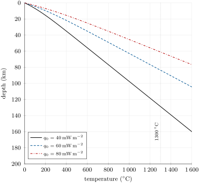
The figure below shows geotherms for surface heat flows of 40, 60 and 80mWm−2, the first typical of cratons and the last of back-arc regions, with k=2.5Wm−1K−1, hr=10km and a crustal share A0hr=0.4q0. The 1300∘C isotherm, taken as the base of the thermal lithosphere, lies at 129, 84 and 61km. Seismology finds cratonic mantle fast down to about 250km, and back-arc lithosphere 50 to 60km thick: the cold, thick roots of cratons need a smaller reduced heat flow than this simple model gives them, and their conductivity changes with temperature, but the order of the contrast is right.
Steady continental geotherms with exponentially decreasing heat production (hr=10km, A0hr=0.4q0, k=2.5Wm−1K−1) for three surface heat flows. The curvature near the surface is the crust’s own heat; below a few depth scales each geotherm is a straight line of gradient qm/k.
In the field— Measuring heat flow at sea
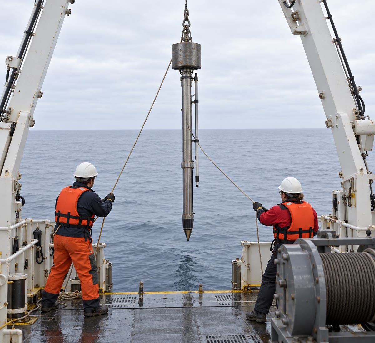
A heat-flow lance about to be lowered from the stern of a research ship (AI-generated illustration).
A marine heat-flow probe is a long steel lance with a heavy weight on top and a slender tube of temperature sensors along its side. From the stern of a research ship it is lowered on the winch cable to the sea floor and lets itself fall into the soft sediment, sensors and all. It stays still for some minutes while the frictional heat of the penetration dies away and the sensors settle to the temperature of the mud around them: their readings, metres apart, give the temperature gradient. A short pulse of heat is then sent along the tube, and the rate at which it decays gives the conductivity of the sediment around it; the product of the two is the heat flow. The lance is pulled out and set down again a few hundred metres further along the line, without coming back on deck.
5.5 Exercises
Exercise 5.1★
With κ=10−6m2s−1, compute the conductive time L2/κ for L=1, 10 and 100km, in millions of years.
Solution
Solution of Exercise 5.1.
L2/κ=1012s, 1014s and 1016s: 0.032, 3.2 and 317Myr. A kilometre forgets its temperature in tens of thousands of years, a hundred kilometres in hundreds of millions.
Exercise 5.2★
A mountain range is eroded at 1mm/yr, and rock rises through the upper 30km of crust to replace it. With κ=10−6m2s−1, compute the Péclet number. Can the geotherm of the range be computed by conduction alone?
Solution
Solution of Exercise 5.2.
u=10−3m/3.156×107s=3.17×10−11ms−1, so Pe=3.17×10−11×3×104/10−6=0.95. Advection and conduction are of the same importance: the rising rock carries heat upwards and steepens the geotherm near the surface, and conduction alone would underestimate the gradient.
Exercise 5.3★
In the half-space model (T0=0, Tm=1450∘C, κ=0.8×10⁻⁶m2s−1), compute the temperature 10km below sea floor 5Myr old (1Myr=3.156×10¹³s; erf0.445=0.471).
Solution
Solution of Exercise 5.3.
κt=0.8×10−6×5×3.156×1013=11236m, η=10000/(2×11236)=0.445, and T=1450×0.471=683∘C.
Exercise 5.4★
With Cq=490mWm−2Myr1/2, compute the heat flow through sea floor 1, 25 and 100Myr old. Which of the three would a probe most likely underestimate?
Solution
Solution of Exercise 5.4.
490/1=490, 490/5=98 and 490/10=49mWm−2. The probe would most likely underestimate the first: young crust is cracked and open to circulating sea water, which carries part of the heat away by hot springs.
Exercise 5.5★★
In the half-space model, the temperature reaches 90% of Tm where erfη=0.9, η=1.163. With κ=0.8×10⁻⁶m2s−1, compute that depth at 10, 40 and 100Myr.
Solution
Solution of Exercise 5.5.
z=2×1.163κt: with κt=15.89, 31.78 and 50.25km, z=37.0, 73.9 and 116.9km. The cooled layer doubles from 10 to 40Myr; by 100Myr it is already deeper than a 95km plate.
Exercise 5.6★★
With the values of the text, the half-space model gives C=370.5mMyr−1/2. Keeping every other value, what thermal expansion coefficient would give the fitted 350mMyr−1/2? What other parameter could be changed instead?
Solution
Solution of Exercise 5.6.
C is proportional to α: α=3.1×10−5×350/370.5=2.93×10−5K−1. C is also proportional to Tm−T0 (a mantle at 1450×350/370.5=1370∘C) and to κ (a diffusivity 0.8×(350/370.5)2=0.71×10−6m2s−1): depth alone cannot separate them, which is why heat flow is used as well.
Exercise 5.7★★
Compute the asymptotic heat flow kTm/L of the plate model for L=95km, Tm=1450∘C, and for L=125km, Tm=1350∘C, with k=3.1Wm−1K−1 in both. Which is closer to the heat flow of old ocean floor computed from Cq/t at 150Myr with Cq=490mWm−2Myr1/2?
Solution
Solution of Exercise 5.7.
3.1×1450/95×103=47.3mWm−2 and 3.1×1350/125×103=33.5mWm−2. The half-space reaches them at (490/47.3)2=107Myr and (490/33.5)2=214Myr: the thin, hot plate holds the heat flow of old floor at 47mWm−2 from about 100Myr on, whereas the thicker, colder one would let it fall below 40mWm−2, the half-space value at 150Myr.
Exercise 5.8★★
A province has q0=60mWm−2, hr=10km and A0hr=0.4q0. Compute A0, qm and the temperature at the Moho, 35km deep, with k=2.5Wm−1K−1.
Solution
Solution of Exercise 5.8.
A0hr=0.4×60=24mWm−2, so A0=24×10−3/104=2.4µWm−3 and qm=60−24=36mWm−2. At 35km, T=36×10−3×35×103/2.5+2.4×10−6×108/2.5×(1−e−3.5)=504+96×0.970=597∘C.
Exercise 5.9★★
Two granite plutons of one province give q0=66mWm−2 with A0=3.0µWm−3, and q0=48mWm−2 with A0=1.2µWm−3. Assuming they lie on the line of Proposition 5.10, compute hr and qm.
Solution
Solution of Exercise 5.9.
hr=Δq0/ΔA0=18×10−3/1.8×10−6=10km, and qm=q0−hrA0=66−30=36mWm−2, since hrA0=104×3.0×10−6Wm−3=30mWm−2.
Exercise 5.10★★★
(a) Show that the heat lost through the sea floor between ages 0 and t, per unit area, is Q(t)=2k(Tm−T0)t/(πκ) in the half-space model. (b) Show that the subsidence is d−dr=αQ/(c(ρm−ρw)), where c=k/(ρmκ) is the specific heat. (c) Check it numerically at 40Myr with the values of the text.
Solution
Solution of Exercise 5.10.
(a) Q(t)=∫0tk(Tm−T0)/πκt′dt′=2k(Tm−T0)t/(πκ). (b) The heat lost is the heat content removed from the column, Q=ρmc∫0∞(Tm−T)dz, and isostasy gives (ρm−ρw)(d−dr)=ρmα∫0∞(Tm−T)dz=αQ/c. (c) c=3.1/(3300×0.8×10−6)=1174Jkg−1K−1; at 40Myr, t=1.262×10¹⁵s and Q=2×3.1×1450×1.262×1015/(π×0.8×10−6)=2.015×1014Jm−2; d−dr=3.1×10−5×2.015×1014/(1174×2270)=2343m, which is 370.540.
Exercise 5.11★★★
In the plate model of the text (τ=36.2Myr, ρmαTmL/(2(ρm−ρw))=3104m), the depth computed with the first Fourier term alone exceeds the full series mainly by the n=3 term. Compute that term’s size at 1, 10 and 20Myr, and the age after which the first term alone is within 10m of the series.
Solution
Solution of Exercise 5.11.
The n=3 term is 3104×(8/π2)×91e−9t/36.2=280e−9t/36.2 metres: 218m at 1Myr, 23m at 10Myr and 1.9m at 20Myr. It falls to 10m when e−9t/36.2=10/280, at t=(36.2/9)ln28=13.4Myr.
Exercise 5.12★★★
(a) Show that, in the geotherm of Proposition 5.10, T(z)≈qmz/k+A0hr2/k for z≫hr. (b) Deduce the depth of the 1300∘C isotherm for q0=40mWm−2, with the values of exercise 8. (c) By how much must qm fall for that depth to reach 250km, the depth of the fast roots of cratons?
Solution
Solution of Exercise 5.12.
(a) For z≫hr, e−z/hr→0. (b) qm=24mWm−2, A0hr2/k=16×10−3×104/2.5=64K, and z=(1300−64)×2.5/24×10−3=128.8km. (c) qm=2.5×1236/250×103=12.4mWm−2: the reduced heat flow must be about halved, as under a craton whose thick, cold root lets little heat in from below.
5.6 Problem: Forty Million Years off the Ridge
Problem 5.1
Weekend problem — the half-space and the plate, the depth of an invented ocean, and the thickness of its plate
Take T0=0, Tm=1450∘C, κ=0.8×10⁻⁶m2s−1, k=3.1Wm−1K−1, α=3.1×10⁻⁵K−1, ρm=3300kgm−3, ρw=1030kgm−3, a ridge 2500m deep, and 1Myr=3.156×10¹³s.
Part I — The half-space.
Compute κt at 10 and 40Myr.
Compute the temperature 20km below the floor at both ages (erf0.6294=0.6266, erf0.3147=0.3437).
The 1000∘C isotherm lies where erfη=0.6897, η=0.7174. Compute its depth at both ages, and the age at which it reaches 60km.
Compute the heat flow at both ages, and Cq.
A ridge spreads at 25mm/yr on each side. Compute the Péclet number of the plate over 95km. Why may each column be cooled alone?
Compute the conductive time across 95km. What does it say of a half-space model of floor 150Myr old?
Part II — Subsidence.
Recall the isostatic balance that turns the temperature deficit of a column into subsidence, and why the integral may be taken to infinity in the half-space.
Compute C of the depth–age law, and the depths at 10 and 40Myr.
The median depth of the real ocean floor between 40 and 45Myr is 4475m, uncorrected. Compare with the model at 42.5Myr, and list what the median includes that the model leaves out.
By how much would C change if Tm were 1350∘C? Compare with the fitted 350mMyr−1/2.
Why do measured heat flows on young floor fall below Cq/t?
Part III — The plate. Take L=95km.
Compute τ and the amplitude ρmαTmL/(2(ρm−ρw)).
Compute the depth at 40Myr with the terms n=1, 3 and 5.
How much does the first term alone differ from that, and why so little?
Compute the difference between the half-space and the plate at 40 and 50Myr, and estimate by linear interpolation the age at which it reaches 100m.
Compute the heat flow of the plate at 40Myr, with the terms n=1 to 3, and compare with the half-space.
Give the asymptotic depth and heat flow.
Part IV — An invented ocean. In an invented ocean whose ridge is 2500m deep, the floor, once corrected for sediment and away from seamounts and swells, is 5700m deep at 120Myr and 4800m at 40Myr. The plate’s L is unknown; every other value is as above.
Keeping the first Fourier term only, write the depth at 120Myr as a function of L, with τ itself depending on L.
Solve it for L by iteration, starting from L=100km: compute τ, then the L that matches 5700m with that τ, and repeat.
With the L found, compute the depth at 40Myr and compare with the half-space and with the 4800m measured.
Compute τ for that L and the asymptotic depth of this ocean.
After what age does the floor lie within 100m of its asymptotic depth?
Give the thickness L of the plate that fits the old floor of the invented ocean.
Solution
Solution of Problem 5.1.
1.0.8×10−6×3.156×1014=15889m and 0.8×10−6×1.2624×1015=31778m.
2.η=20000/31778=0.6294 and 20000/63556=0.3147: T=1450×0.6266=909∘C at 10Myr and 1450×0.3437=498∘C at 40Myr.
3.z=2×0.7174κt: 22.8km and 45.6km. It reaches 60km when κt=60/1.4348=41.82km, at t=(41.82×10³)2/0.8×10−6=2.186×1015s, 69.3Myr.
4.q=3.1×1450/(π×15889)=159.6mWm−2 at 10Myr and 79.8mWm−2 at 40Myr; Cq=159.610=505mWm−2Myr1/2.
5.u=7.92×10⁻¹⁰ms−1, Pe=7.92×10−10×95×103/0.8×10−6=94. Heat travels sideways with the plate a hundred times faster than it diffuses sideways, so each column cools by vertical conduction only.
6.(95×103)2/0.8×10−6=1.13×1016s, 357Myr. At 150Myr, κt=61.5km and the cooled layer, a few times that, reaches far below 95km: a half-space model of so old a floor assumes that cold has reached depths where the mantle convects.
7.(ρm−ρw)(d−dr)=ρmα∫(Tm−T)dz, the masses of the ridge column and of the old column being equal above a compensation depth. Tm−T=Tmerfcη falls below 0.5% of Tm for η>2, so the deep part adds nothing.
8.C=2×3300×3.1×10−5×1450/2270×0.8×10−6×3.156×1013/π=0.13069×2834.8=370.5mMyr−1/2; d=2500+370.510=3672m and 2500+370.540=4843m.
9. The model gives 2500+370.542.5=4915m, 440m deeper than the median. The median includes the load of the sediment, the seamounts and volcanic plateaus, the swells of hotspots, and cells on the flanks of fracture zones and margins, all of which make the floor shallower.
10.C is proportional to Tm: 370.5×1350/1450=344.9mMyr−1/2, close to the fitted 350.
11. Sea water circulating through the cracked young crust carries part of the heat out through hot springs, between the probes.
12.τ=(95×103)2/(π2×0.8×10−6)=1.143×1015s=36.2Myr; the amplitude is 3300×3.1×10−5×1450×95×103/4540=3104m.
13.e−40/36.2=0.33124, e−360/36.2/9=5.3×10−6 and the n=5 term is smaller still; the bracket is 1−0.81057×0.33125=0.73150, and d=2500+3104×0.73150=4771m.
14. By the n=3 term, 3104×0.81057×5.3×10−6=0.013m: at 40Myr, e−9t/τ is 10−4 of e−t/τ, and only the first mode is left.
15. At 40Myr, 4843−4771=73m; at 50Myr, 2500+370.550=5120 against 2500+3104×(1−0.81057×0.25127)=4972: 148m. Interpolating, 40+10×(100−73)/(148−73)=43.6Myr, about 44Myr (the full series gives 44.0).
16.q=(3.1×1450/95×103)[1+2(0.33124+0.01204+0.00005)]=47.32×1.68666=79.8mWm−2, the same as the half-space: at 40Myr the base has not yet made itself felt at the surface.
17.2500+3104=5604m and kTm/L=47.3mWm−2.
18.d(120)=2500+aL[1−(8/π2)e−120/τ], with a=ρmαTm/(2(ρm−ρw))=32.673m/km and τ=L2/(π2κ).
19.L=3200/(32.673[1−0.81057e−120/τ]). From L=100km: τ=40.13Myr, bracket 0.95925, L=102.10km; then τ=41.83, L=102.67; τ=42.30, L=102.82; τ=42.43, L=102.87; it settles at L=102.9km.
20.τ=42.48Myr, aL=3362m: d(40)=2500+3362×(1−0.81057e−40/42.48)=4799m, against 4843m for the half-space and 4800m measured: the plate fits both ages.