University Earth and Space Sciences — Year 3 · 本科三年级
19Geophysical Fluid Dynamics
Stir a cup of tea and the swirl dies in a minute; the leaves gather in the middle of the bottom and nothing else happens. The ocean and the atmosphere are stirred too, by the Sun and the wind, but on a rotating planet and in layers of different density. Rotation and stratification make them obey rules that a teacup never shows: winds blow along the isobars instead of across them, columns of fluid refuse to tilt, and the wind of the upper troposphere is written in the temperatures below it. This chapter sets up the equations of these large, slow, thin flows and the few numbers that decide which terms matter.
You already know
The Coriolis and centrifugal forces in a rotating frame, the Navier–Stokes and continuity equations, viscosity, the Reynolds number and the hydrostatic relation are in the physics books. The Coriolis parameter f=2Ωsinφ, the pressure-gradient force, geostrophic balance, the geostrophic and gradient winds and the jet streams are in the Year 1 volume, in its chapter on the general circulation of the atmosphere; the Ekman layer in its chapter on the circulation of the ocean; potential temperature, static stability and the oscillation of a lifted air parcel in its chapter on the structure of the atmosphere and the ocean.
19.1 Equations in a rotating frame
In a frame that turns with the Earth at the angular velocity Ω, a fluid parcel of velocity u obeys
DtDu+2Ω×u=−ρ1∇p+g+ν∇2u,∂t∂ρ+∇⋅(ρu)=0,
where D/Dt=∂/∂t+u⋅∇ is the derivative following the parcel and ν the kinematic viscosity. The centrifugal force has been added to gravitation: their sum g is the effective gravity, normal to the level surfaces of the geopotential, and the vertical is defined by it. Only the Coriolis term, −2Ω×u, remains of the rotation, and it does no work: it turns a parcel without changing its speed. The Earth turns at Ω=7.292115×10⁻⁵rad/s, once a sidereal day of 23.9345h.
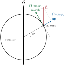
For motion over distances much smaller than the Earth’s radius a, a local Cartesian frame is enough: x eastward, y northward, z upward, at the latitude φ, the tangent plane of the figure below. There Ω=Ω(0,cosφ,sinφ), and the three components of the momentum equation are
with F the friction. For the thin, nearly horizontal flows of the ocean and the atmosphere the terms in f~ are dropped: f~w is small beside fv because w≪v, and f~u is a ten-thousandth of g (Exercise 19.5). The Coriolis force then acts only in the horizontal, through the local vertical component of the rotation, Ωsinφ.
Definition 19.1(f-plane and β-plane)
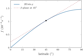
Near a reference latitude φ0, the f-plane approximation takes the Coriolis parameter as constant, f=f0=2Ωsinφ0. The β-plane approximation keeps its first-order change with the northward distance y: f=f0+βy, with β=df/dy=2Ωcosφ0/a.
At 45∘, with the mean radius a=6371km, f0=1.031×10⁻⁴s−1 and β=1.62×10⁻¹¹m−1s−1: over 1000km of latitude f changes by 16%. The f-plane suits motions much smaller than that; the β-plane is needed for basin-wide currents and planetary waves.
Left, the local frame at latitude φ: z along the local vertical, y northward in the tangent plane, x eastward into the page. The rotation vector splits into Ωsinφ about the vertical, which turns horizontal motion, and Ωcosφ about the northward axis, dropped for thin flows. Right, the Coriolis parameter and its β-plane tangent at 45∘: close over a band of latitude, far from it near the equator and the pole.
Two more approximations simplify the equations without losing what matters. The first concerns density.
Definition 19.2(Boussinesq approximation)
The Boussinesq approximation writes the density as ρ=ρ0+ρ′, with ρ0 a constant and ∣ρ′∣≪ρ0, and keeps ρ′ only where it is multiplied by g. The continuity equation becomes ∇⋅u=0, and the momentum equation
DtDu+fk×u=−ρ01∇p′+bk+ν∇2u,b=−gρ0ρ′,
where p′ is the departure of the pressure from the hydrostatic pressure of the density ρ0, k the upward unit vector and b the buoyancy.
In the ocean ρ′ is a few kg/m3 on 1025, a fraction of a per cent, and the approximation is excellent. In the atmosphere density falls by a factor e in about 8.5km; the approximation holds for layers much thinner than that, and deeper flows replace ρ0 by a mean profile ρ0(z), with the same physics.
The second concerns the vertical. A fluid at rest is in hydrostatic equilibrium; a fluid in motion keeps it to a very good approximation when the motion is much wider than it is deep.
Definition 19.3(Hydrostatic approximation)
The hydrostatic approximation replaces the vertical momentum equation of a moving fluid by the hydrostatic relation, ∂p/∂z=−ρg.
Proposition 19.4(When the hydrostatic approximation holds)
For a motion of horizontal scale L, depth H and speed U, with a Rossby numberU/(fL) at most of order one, the vertical acceleration is smaller than the vertical gradient of the pressure perturbation by a factor of order (U/fL)(H/L)2.
Proof. When the Coriolis force is at least as large as the acceleration, the horizontal momentum equation balances the horizontal pressure gradient against it: p′/(ρ0L)∼fU, so p′/ρ0∼fUL, and the vertical gradient is p′/(ρ0H)∼fUL/H. Continuity, ∂w/∂z=−(∂u/∂x+∂v/∂y), bounds the vertical velocity by W∼UH/L, and the vertical acceleration by Dw/Dt∼UW/L=U2H/L2. The ratio is (U2H/L2)/(fUL/H)=(U/fL)(H/L)2. ∎
A weather system 1000km wide in a troposphere 10km deep has (H/L)2=10−4 and a Rossby number of about 0.1: the error of the hydrostatic approximation is of order 10−5. It fails only in narrow, deep motions: a thunderstorm updraught, a convective plume in the ocean.
19.2 Scales of rotating flow
Which terms of the momentum equation matter is decided by two ratios.
Definition 19.5(Rossby and Ekman numbers)
For a flow of speed U, horizontal scale L and depth H on a planet of Coriolis parameter f, the Rossby number is Ro=U/(fL), the ratio of the acceleration, of order U2/L, to the Coriolis force, of order fU. The Ekman number is Ek=ν/(fH2), the ratio of the viscous force, of order νU/H2, to the Coriolis force; in a turbulent flow ν is replaced by an eddy viscosity.
A bathtub draining 0.1m/s over 0.3m has a Rossby number of some thousands: the Earth’s rotation does not decide the sense of its swirl. A depression 1000km across with winds of 15m/s has Ro≈0.14, and an ocean gyre Ro∼10−4. Viscosity is weaker still: the molecular viscosity of water is 10−6m2/s, and the eddy viscosities that stand for the turbulence of the ocean, 10−5 to 10−3m2/s in the vertical, give Ek∼10−5 over 1000m of depth. The two numbers are related to the Reynolds number by Re=UL/ν=(Ro/Ek)(L/H)2.
When both numbers are small, the steady horizontal momentum equation keeps only the Coriolis force and the pressure gradient: the flow is in geostrophic balance, fk×ug=−(1/ρ)∇hp, which the Year 1 volume read from weather maps. Geostrophy is the limit Ro,Ek→0; its corrections are of order Ro, and friction acts only in thin layers of relative thickness Ek, the Ekman layers at the bottom of the atmosphere and the top and bottom of the ocean. On an f-plane the geostrophic velocity has no horizontal divergence: ∂ug/∂x+∂vg/∂y=−(1/ρf)(∂2p/∂x∂y−∂2p/∂y∂x)=0 for uniform ρ.
The opposite limit, rotation with no pressure gradient, is the simplest motion a rotating fluid can make.
Definition 19.6(Inertial oscillation)
An inertial oscillation is the horizontal motion of a fluid on which no horizontal force acts but the Coriolis force.
Theorem 19.7(Inertial circles)
On an f-plane, a parcel set moving at speed U with no horizontal force but the Coriolis force keeps its speed and describes a circle of radius U/∣f∣, clockwise in the Northern Hemisphere and anticlockwise in the Southern, in the inertial period 2π/∣f∣, which is half a sidereal day divided by sinφ.
Proof. The equations are du/dt=fv, dv/dt=−fu. With w=u+iv they read dw/dt=−ifw, so w=Ue−ift for a start eastward: the speed ∣w∣=U is constant and the velocity turns at the rate f, clockwise when f>0. Integrating, the position x+iy=(iU/f)(e−ift−1) runs round the point −iU/f at the distance U/∣f∣. The period is 2π/∣f∣=2π/(2Ω∣sinφ∣), and 2π/Ω is the sidereal day. ∎
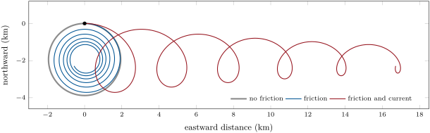
At 45∘ the inertial period is 16.9h, and a current of 0.2m/s turns on a circle of 1.94km; at 30∘ the period is a full sidereal day, and at the equator there are no inertial circles. After a storm has set the surface layer of the ocean moving and then died, the water does exactly this. Drogued drifting buoys at 15m in the North Pacific traced loops for days after a storm in October 1987, carried along by the mean current: the third path of the figure below, after the circle and the spiral.
Paths over four days of a parcel set moving eastward at 0.2m/s at 45∘ N (dot), with no force but the Coriolis force: a circle of radius 1.94km run clockwise every 16.9h (grey); with a friction that halves the speed in 2.8 days, an inward spiral (blue); the same carried by a steady eastward current of 0.05m/s, a train of shrinking loops (red).
Between geostrophy and the inertial circle lies the flow round a centre of high or low pressure, where the isobars are curved and the acceleration towards the centre is no longer negligible.
Definition 19.8(Gradient wind)
The gradient wind is the steady, frictionless flow along curved isobars in which the pressure-gradient force, the Coriolis force and the centripetal acceleration balance.
Proposition 19.9(The curvature correction)
Let the isobars be circles of radius r in the Northern Hemisphere, and Vg the geostrophic speed that their pressure gradient would give, with Rog=Vg/(fr). Round a low, the gradient wind is V=2Vg/(1+1+4Rog), slower than Vg; round a high, V=2Vg/(1+1−4Rog), faster, and it exists only if Rog≤1/4. To first order, V=Vg(1∓Rog).
Proof. Round a low the wind turns anticlockwise; the pressure-gradient force fVg points to the centre, the Coriolis force fV outward, and their difference provides the centripetal acceleration: fVg−fV=V2/r. The positive root of V2+frV−frVg=0 is V=(fr/2)(1+4Rog−1); multiplying by (1+4Rog+1)/(1+4Rog+1) gives the formula. Round a high, the wind turns clockwise and the Coriolis force points inward: fV−fVg=V2/r, so V2−frV+frVg=0, which has real roots only if f2r2≥4frVg; the root that tends to Vg when Rog→0 is V=(fr/2)(1−1−4Rog). Expanding the square roots, V=Vg(1∓Rog+…). ∎
The Rossby number of the isobars measures the correction: a tenth for a depression of moderate size. The condition Rog≤1/4 is why the centre of an anticyclone has weak gradients and light winds, while that of a depression can hold steep gradients and gales.
19.3 Rotation without stratification
A rotating fluid of uniform density, in slow motion, behaves as if it were made of rigid columns parallel to the rotation axis.
Theorem 19.10(Taylor–Proudman)
In a steady flow of an inviscid fluid of uniform density, rotating at Ω, with small Rossby number, the velocity does not vary along the direction of the rotation axis: (Ω⋅∇)u=0.
Proof. For Ro→0, steady and inviscid, the momentum equation reduces to 2Ω×u=−∇(p/ρ0+Φ), with Φ the geopotential. The curl of a gradient vanishes, so ∇×(Ω×u)=0. For a constant Ω this curl is Ω(∇⋅u)−(Ω⋅∇)u, and ∇⋅u=0 for uniform density. ∎
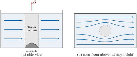
With Ω along z, ∂u/∂z=0: all three velocity components are the same at every height. If a rigid bottom forbids w there, w=0 everywhere, and the horizontal flow is the same at every level. An obstacle on the floor of a rotating tank is therefore felt all the way to the surface: the fluid above it cannot climb over it, since that would stretch or squeeze a column, and goes round it at every height. The column of fluid that stays above the obstacle is a Taylor column.
A Taylor column (schematic). (a) In a tank of uniform water rotating rapidly, a slow flow meets a low obstacle on the floor; the fluid above the obstacle (grey) is held in place up to the surface, and the flow at every height goes round the column as if the obstacle reached the top. (b) The flow seen from above is the same at every level.
The atmosphere and the ocean are stratified, and stratification relaxes the constraint: a stratified fluid can vary with height, in the way the thermal wind theorem prescribes.
19.4 Stratification and the thermal wind
The Year 1 volume lifted an air parcel in a stable atmosphere and found that it oscillates about its level. The same holds in any stratified fluid, and the frequency of the oscillation is the measure of stratification.
Definition 19.11(Buoyancy frequency)
The buoyancy frequencyN of a fluid at rest is defined by
N2=θgdzdθ(air),N2=−ρ0gdzdρθ(seawater),
where θ is the potential temperature of the air and ρθ the potential density of the water, the density it would have if brought adiabatically to a reference pressure.
Theorem 19.12(Oscillation of a displaced parcel)
A parcel displaced vertically by a small distance ζ from its level in a fluid at rest, adiabatically and without mixing, obeys ζ¨=−N2ζ. If N2>0 it oscillates at the angular frequency N; if N2<0 the displacement grows and the fluid is unstable.
Proof. Moved adiabatically and without mixing, the parcel keeps its potential density ρθ(z0). At the level z0+ζ it is at the pressure of its surroundings, whose potential density is ρθ(z0)+ζdρθ/dz; two parcels at the same pressure differ in density by the difference of their potential densities, to first order. The buoyancy force per unit mass is −g(ρp−ρe)/ρ0=gζ(dρθ/dz)/ρ0=−N2ζ. For air at a given pressure the density varies as 1/θ, so −dρθ/ρ0=dθ/θ and the two forms of N2 agree. ∎
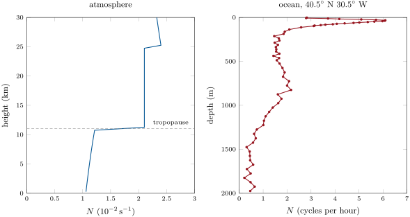
In the troposphere of the standard atmosphere, which cools by 6.49K/km against the 9.77K/km of the dry adiabat (g/cp, with cp=γR/(γ−1), γ=1.4 and R=286.9Jkg−1K−1), N averages 0.0113s−1, a period of 9.3min; in the isothermal lower stratosphere it is 0.0210s−1. In the ocean, the water column of the North Atlantic at 40.5∘ N, 30.5∘ W in the annual mean has its strongest stratification in the seasonal pycnocline, N=0.0106s−1 at about 30m, six cycles per hour, and much weaker values below: a few cycles per hour at most, as observed across the upper ocean.
Buoyancy frequency. Left, the standard atmosphere: nearly uniform in the troposphere, twice as large in the isothermal lower stratosphere, larger still above 25km where the temperature rises. Right, an annual-mean column of the North Atlantic (temperature and salinity from the World Ocean Atlas 2023, potential density from EOS-80): a sharp maximum in the seasonal pycnocline, weak stratification below.
Stratification lets the flow vary with height, and how it does so depends on whether the surfaces of constant density follow those of constant pressure.
Definition 19.13(Barotropic and baroclinic fluids)
A fluid is barotropic if its density is a function of pressure alone, so that surfaces of constant density coincide with surfaces of constant pressure; it is baroclinic if they cross.
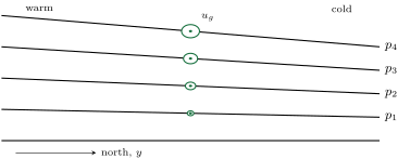
In the atmosphere, a horizontal gradient of temperature along a pressure surface makes the air baroclinic. Hydrostatic balance then makes the pressure surfaces slope more steeply with height, and geostrophic balance turns the growing slope into a growing wind.
The geometry of the thermal wind (schematic, a meridional section with the warm side to the south, p1>p2>p3>p4). Warm air expands, so the layer between two pressure surfaces is thicker on the warm side than on the cold: each surface slopes down towards the cold side more steeply than the one below. The geostrophic wind is proportional to the slope, and grows with height (circles, larger for stronger wind), eastward, out of the page.
Theorem 19.14(Thermal wind)
In an atmosphere in hydrostatic and geostrophic balance, the geostrophic wind varies with pressure as
∂lnp∂ug=fR(∂y∂T)p,∂lnp∂vg=−fR(∂x∂T)p.
Between two pressure levels pb>pt, the thermal wind, the difference of the geostrophic winds, is
ug(pt)−ug(pb)=fRlnptpbk×∇pTˉ,
where Tˉ is the mean temperature of the layer: it blows along the isotherms of the layer with the cold air on its left in the Northern Hemisphere.
Proof. On a surface of constant pressure, dp=(∂p/∂y)dy+(∂p/∂z)dz=0, and with ∂p/∂z=−ρg the height zp of the surface satisfies g∂zp/∂y=(1/ρ)∂p/∂y. In terms of the geopotentialΦ=gzp of the surface, geostrophic balance reads fug=−∂Φ/∂y and fvg=∂Φ/∂x, with the derivatives taken along the surface. The hydrostatic relation and the ideal gas law give ∂Φ/∂p=−1/ρ=−RT/p, that is ∂Φ/∂lnp=−RT. Differentiating fug=−∂Φ/∂y with respect to lnp gives f∂ug/∂lnp=R∂T/∂y, and likewise for vg. Integrating from pb to pt, lnp decreases by ln(pb/pt), so ug(pt)−ug(pb)=−(R/f)ln(pb/pt)∂Tˉ/∂y, and vg(pt)−vg(pb)=(R/f)ln(pb/pt)∂Tˉ/∂x: these are the components of the vector form, since k×∇Tˉ=(−∂Tˉ/∂y,∂Tˉ/∂x). ∎
Corollary 19.15(Thermal wind in height)
In height coordinates, for the atmosphere, ∂ug/∂z=−(g/fT)∂T/∂y+(ug/T)∂T/∂z; for the ocean in the Boussinesq approximation, ∂ug/∂z=(g/fρ0)∂ρ/∂y and ∂vg/∂z=−(g/fρ0)∂ρ/∂x.
Proof. In the air, fug=−(1/ρ)∂p/∂y=−RT∂lnp/∂y and ∂lnp/∂z=−g/(RT). Then
f∂z∂(ug/T)=−R∂y∂∂z∂lnp=g∂y∂(1/T)=−T2g∂y∂T,
and expanding the left side gives the formula. In the ocean, fug=−(1/ρ0)∂p/∂y and ∂p/∂z=−ρg, so f∂ug/∂z=(g/ρ0)∂ρ/∂y; likewise for vg. ∎
The second term of the atmospheric form, from the decrease of temperature with height, is smaller than the first and vanishes in an isothermal layer; integrated across a layer with its mean temperature, the first term alone gives nearly the pressure form, since Δz≈(RTˉ/g)ln(pb/pt) (Problem, Part IV). In the ocean the same theorem turns a section of density across a current into its vertical shear: the basis of the dynamic method of the oceanographers.
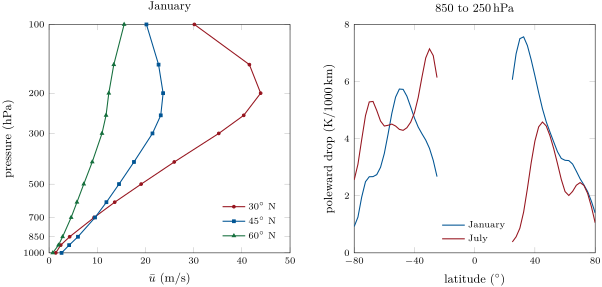
The jet streams of the Year 1 volume are thermal winds. In the January zonal mean of 1991–2020, the westerly wind at 30∘ N grows from 4.3m/s at 850hPa to 40.4m/s at 250hPa; with f at 30∘ and R, this shear is the signature of a layer whose mean temperature falls northward by 7.5K per 1000km. At 45∘ N the shear from 6.0 to 23.2m/s gives 5.0K per 1000km. The figure below shows the profiles and, for each latitude, the poleward drop of temperature read from the shear: largest in the subtropics of the winter hemisphere, which is where the subtropical jet stands, 43.9m/s at 200hPa and 30∘ N in January and 41.0m/s at 30∘ S in July. Above 200hPa at 30∘ N the wind weakens again: the thermal wind theorem read backwards says that there, in the lower stratosphere, the temperature rises towards the pole.
Left, zonal-mean zonal wind in January (NCEP–NCAR Reanalysis 1, 1991–2020 mean) at three latitudes: the wind grows with height through the troposphere. Right, the layer-mean temperature drop towards the pole between 850hPa and 250hPa read from the wind shear by the thermal wind theorem (equatorward of 25∘, where geostrophy fails, left out): larger in the winter hemisphere.
19.5 The Rossby radius of deformation
Rotation and stratification each impose a scale; together they impose a length.
Definition 19.16(Rossby radius of deformation)
The Rossby radius of deformation of a layer of depth H and buoyancy frequencyN is LR=NH/∣f∣.
Proposition 19.17(Potential and kinetic energy of balanced flow)
In a hydrostatic, geostrophic flow of horizontal scale L in a layer of depth H and buoyancy frequencyN, the ratio of the potential energy stored in the displaced density surfaces to the kinetic energy is of order (L/LR)2.
Proof. Geostrophy gives the pressure perturbation p′/ρ0∼fUL; the hydrostatic relation gives the buoyancy b∼p′/(ρ0H)∼fUL/H. A buoyancy b in a fluid of buoyancy frequencyN means density surfaces displaced vertically by η=b/N2, which store a potential energy per unit mass of order N2η2=b2/N2∼f2U2L2/(N2H2). Divided by the kinetic energy, of order U2, this is (fL/NH)2=(L/LR)2. ∎
Motions much wider than LR hold most of their energy in tilted density surfaces, motions much narrower in their velocity; at LR the two are equal, and the instability of baroclinic flows, which feeds on the potential energy of the tilted surfaces, grows fastest near that scale. For the troposphere, with the mean N of the standard atmosphere, H=11km and f at 45∘, LR=1210km: the scale of the depressions and anticyclones on a weather map. For the upper kilometre of the North Atlantic column at 40.5∘ N, LR=38km, thirty times smaller: the ocean has its own weather, eddies tens of kilometres across, and a model that resolves them needs a much finer grid. On scales near LR, f changes by βLR/f, 19% for the atmosphere and under one per cent for the ocean: ocean eddies live on an f-plane, weather systems feel the β-plane.
In the lab— A planet on a turntable
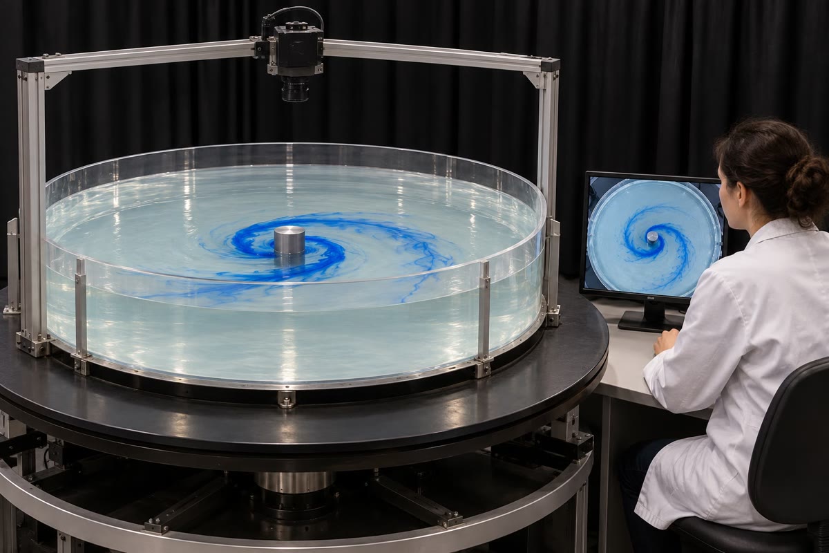
A rotating tank: dye spiralling round a cylinder, filmed by a camera that turns with the table (AI-generated illustration).
In a laboratory of geophysical fluid dynamics, a tank of water stands on a turntable; a camera turns with it and sees the water as an observer on a planet would. Before each run the water is left to spin up until it turns as a solid body, which takes a few minutes, many turns of the table. Then the experimenters inject dye, or move an obstacle slowly along the floor: the dye rises in a vertical column above the obstacle and the flow parts round it at every level. With a layer of fresh water over salt water, or a heated outer wall and a cooled centre, the tank becomes baroclinic, and jets, eddies and meandering fronts appear, whose size the Rossby radius of the tank predicts.
19.6 Exercises
Exercise 19.1★
Take Ω=7.292115×10⁻⁵rad/s. (a) Compute the Coriolis parameter and the inertial period at 30∘, 45∘ and 60∘ N. (b) Compute the radius of the inertial circle of a current of 0.20m/s at the same latitudes. (c) Compare the inertial period at 30∘ with the sidereal day, 23.9345h.
Solution
Solution of Exercise 19.1.
(a) f=2Ωsinφ: 7.292×10⁻⁵, 1.031×10⁻⁴ and 1.263×10⁻⁴s−1; 2π/f: 23.93, 16.92 and 13.82h. (b) U/f: 2.74, 1.94 and 1.58km. (c) At 30∘, sinφ=1/2 and 2π/f=2π/Ω: the inertial period is the sidereal day, 23.93h.
Exercise 19.2★
At 45∘ N, compute the Rossby number of a dust devil (10m/s, 10m), a sea breeze (5m/s, 20km), a depression (15m/s, 1000km) and an ocean gyre (0.05m/s, 2000km). Which of them are close to geostrophic balance?
Solution
Solution of Exercise 19.2.
With f=1.031×10⁻⁴s−1: dust devil 9.7×10³, sea breeze 2.4, depression 0.15, gyre 2.4×10⁻⁴. The depression and the gyre are close to geostrophic balance; the dust devil turns either way, unaware of the Earth’s rotation, and the sea breeze feels it only over a day.
Exercise 19.3★
At 45∘ N the mean temperature of the troposphere, 250K, falls northward by 5K per 1000km. Using the first term of the thermal wind in height, compute the vertical shear of the westerly wind and the increase of the wind over 10km.
Solution
Solution of Exercise 19.3.
∂ug/∂z=(g/fT)∣∂T/∂y∣=9.81×5×10−6/(1.031×10−4×250)=1.90×10−3s−1; over 10km the westerly wind increases by 19m/s.
Exercise 19.4★
The stability E=−(1/ρ)dρθ/dz of the upper kilometre of the ocean lies between 50×10−8 and 1000×10−8m−1; in deep trenches it is 10−8m−1. Compute N=gE, the period of the buoyancy oscillation and N in cycles per hour for these three values.
Solution
Solution of Exercise 19.4.
E=50×10−8: N=2.21×10⁻³s−1, a period of 47min, 1.27 cycles per hour. E=1000×10−8: N=9.90×10⁻³s−1, 10.6min, 5.7 cycles per hour. E=10−8: N=3.13×10⁻⁴s−1, 5.6h, 0.18 cycles per hour.
Exercise 19.5★★
A weather system has U=10m/s, L=1000km, H=10km, at 45∘ N. (a) Estimate its vertical velocity and its vertical acceleration, and compare the latter with g and with the vertical gradient of the pressure perturbation, fUL/H. (b) Compute the dropped Coriolis term f~u and compare it with g.
Solution
Solution of Exercise 19.5.
(a) W∼UH/L=0.1m/s and Dw/Dt∼UW/L=10−6m/s2, 1.0×10⁻⁷ of g. The pressure term, fUL/H=0.103m/s2, is larger by 1×10⁵: the ratio, 9.7×10⁻⁶, is Ro(H/L)2 with Ro=0.097. (b) f~u=2Ωcos45∘×10=1.03×10⁻³m/s2, 1.05×10⁻⁴ of g.
Exercise 19.6★★
Take f=10−4s−1 and circular isobars of radius 300km. (a) The pressure gradient round a low gives Vg=20m/s: compute the gradient wind. (b) Round a high, Vg=5m/s: compute the gradient wind. (c) What is the largest Vg possible round the high, and the wind then?
Solution
Solution of Exercise 19.6.
fr=30m/s. (a) Rog=0.667, V=40/(1+3.667)=13.7m/s, a third slower than geostrophy. (b) Rog=0.167, V=10/(1+0.333)=6.34m/s. (c) Vg≤fr/4=7.5m/s, and then V=fr/2=15m/s, twice the geostrophic speed.
Exercise 19.7★★
A tank 20cm deep turns once every 6s; its water has ν=10−6m2/s. (a) Compute f=2Ω, then the Rossby number of a flow of 1cm/s past a cylinder 5cm across, and the Ekman number of the tank. Will a Taylor column form? (b) Theory gives a spin-up time H/νΩ: compute it in minutes and in turns of the table.
Solution
Solution of Exercise 19.7.
(a) Ω=2π/6=1.047rad/s, f=2.094s−1. Ro=0.01/(2.094×0.05)=0.095 and Ek=10−6/(2.094×0.04)=1.19×10−5: both small, so the flow obeys the Taylor–Proudman theorem and a Taylor column forms. (b) 0.2/10−6×1.047=195s, 3.3min, 33 turns of the table.
Exercise 19.8★★
In the January zonal mean of 1991–2020 the westerly wind is 4.27m/s at 850hPa and 40.39m/s at 250hPa at 30∘ N, 5.99m/s and 23.17m/s at 45∘ N. With R=286.9Jkg−1K−1, compute the meridional gradient of the layer-mean temperature at both latitudes, and say why the jet is stronger at 30∘ N.
Solution
Solution of Exercise 19.8.
∂Tˉ/∂y=−fΔu/(Rln(850/250)), with ln(850/250)=1.224. At 30∘ N, −7.29×10−5×36.12/(286.9×1.224)=−7.50K per 1000km; at 45∘ N, −1.031×10−4×17.18/351.1=−5.05K per 1000km. The shear is proportional to the gradient divided by f: the gradient is 1.5 times larger at 30∘ and f 1.4 times smaller, so the shear is 2.1 times larger.
Exercise 19.9★★
(a) Compute the Rossby radius of the troposphere (N=0.0113s−1, H=11km, 45∘ N) and of the upper ocean (N=0.00357s−1, H=1000m, 40.5∘ N). (b) With a=6371km, compute β at both latitudes and the relative change βLR/f of the Coriolis parameter over each radius.
Solution
Solution of Exercise 19.9.
(a) LR=0.0113×11000/1.031×10−4=1206km; 0.00357×1000/9.47×10−5=37.7km, 32 times smaller. (b) β=2Ωcosφ/a: 1.62×10⁻¹¹ and 1.74×10⁻¹¹m−1s−1. βLR/f=0.19 for the atmosphere, 0.007 for the ocean.
Exercise 19.10★★★
A parcel of the surface ocean set moving at U is slowed by a linear friction: du/dt=fv−ru, dv/dt=−fu−rv. (a) Solve with w=u+iv and describe the path. (b) The parcel is also carried by a steady current u0 eastward: give its position. (c) At 45∘ N with U=0.2m/s, r−1=4 days and u0=0.05m/s, give its speed relative to the current after four days and the distance it has drifted.
Solution
Solution of Exercise 19.10.
(a) dw/dt=−(r+if)w, so w=Ue−rte−ift: the velocity turns at the rate f while its magnitude decays as e−rt. The position x+iy=U(1−e−(r+if)t)/(r+if) spirals into the point U/(r+if). (b) x+iy=U(1−e−(r+if)t)/(r+if)+u0t: the spiral is drawn out into loops. (c) 0.2e−1=0.074m/s; the centre has drifted u0t=0.05×4×86400=17.3km eastward.
Exercise 19.11★★★
Across an ocean front at 40∘ N the density of the water increases northward by 1kg/m3 over 100km, through the upper 1000m; below, the water is uniform and still. With ρ0=1025kg/m3, compute the vertical shear of the current and the current at the surface. In which direction does it flow?
Solution
Solution of Exercise 19.11.
f=9.37×10⁻⁵s−1; ∂u/∂z=(g/fρ0)∂ρ/∂y=9.81×10−5/(9.37×10−5×1025)=1.02×10−3s−1. With u=0 at 1000m the surface current is 1.02m/s, eastward: in the Northern Hemisphere the current flows with the light water on its right.
Exercise 19.12★★★
The annual-mean column at 40.5∘ N, 30.5∘ W has potential densities σθ=ρθ−1000kg/m3 of 26.029 at the surface, 26.697 at 100m, 27.079 at 500m and 27.628 at 1000m. (a) Compute N in each of the three layers, in s−1 and in cycles per hour. (b) Which layer is the most stable, and why? (c) Compare the values with the range of the upper ocean in Exercise 19.4.
Solution
Solution of Exercise 19.12.
(a) N2=(g/ρ)Δσθ/Δz. 0–100m: 9.81×0.668/(1026.4×100), N=7.99×10⁻³s−1, 4.6 cycles per hour; 100–500m: 3.02×10⁻³s−1, 1.7 cycles per hour; 500–1000m: 3.24×10⁻³s−1, 1.9 cycles per hour. (b) The top 100m: it contains the warm surface water above the seasonal pycnocline. Between 100 and 500m the water is more uniform than below. (c) E=N2/g is 650×10−8, 93×10−8 and 107×10−8m−1, all within the range of the upper ocean.
19.7 Problem: Winds over the Steppe of Orrin
Problem 19.1
Weekend problem — the rotation, the stratification and the winds of an invented plain at 48∘ N
The Steppe of Orrin is a flat plain at 48∘ N with a lake, Lake Orrin, 12km wide, and a small laboratory with a rotating tank. Take Ω=7.292115×10⁻⁵rad/s, g=9.81m/s2, R=286.9Jkg−1K−1 and cp=1004Jkg−1K−1. All values of the steppe, its lake and its winds are invented.
Part I — Does rotation matter?
Compute the Coriolis parameter and the inertial period at Orrin.
Compute the Rossby number of five flows: water draining from a bathtub (0.1m/s over 0.3m); the tank of the laboratory, which turns once every 10s (with f=2Ωtank; 5mm/s over 0.2m); the evening breeze off the lake (5m/s, 20km); a depression (15m/s, 1000km); the gyre of an ocean basin at the same latitude (0.05m/s, 2000km).
Which of these flows feel the rotation that drives them, and which are close to geostrophic?
Compute the Ekman number of the tank (0.2m deep, ν=10−6m2/s), of the depression (eddy viscosity 10m2/s, depth 10km) and of the gyre (eddy viscosity 10−3m2/s, depth 1000m).
The Ekman layer has the thickness δ=2ν/f. Show that δ/H=2Ek and compute δ for the tank and for the air of the steppe.
What do these numbers say about where friction matters?
Part II — The wind at the ground.
At the ground the pressure is 1012.9hPa and the temperature 288.1K. Compute the density of the air.
The sea-level pressure falls northward by 4hPa per 300km. Compute the geostrophic wind and give its direction.
The same gradient surrounds a depression whose isobars have a radius of 600km. Compute the Rossby number of the isobars and the gradient wind.
The same gradient surrounds an anticyclone of the same radius. Compute the gradient wind, and the largest pressure gradient, in hPa per 300km, that the anticyclone can hold.
Part III — Stratification.
The temperature of the troposphere falls by 6.49K/km. Compute the dry adiabatic lapse rate g/cp, and N and the period of the buoyancy oscillation at 5km, where the temperature is 255.7K.
Above 11km the air is isothermal at 216.6K. Show that N2=g2/(cpT) there, and compute N and its ratio to the value of question 11.
Compute the Rossby radius of the troposphere of Orrin, with the N of question 11 and H=10km, and compare it with the size of the depression of Part I.
In summer, the upper 20m of Lake Orrin are lighter than the deep water by 1.5kg/m3 (ρ0=1000kg/m3). Compute the reduced gravity g′=gΔρ/ρ0, the speed g′h of the slow internal waves of the upper layer, and the Rossby radius g′h/f.
Will the rotation of the Earth shape the internal motions of the lake?
Part IV — The thermal wind.
Two radiosonde stations stand 600km apart on the same meridian. The mean temperature of the layer from the ground, 1013hPa, to 265hPa, about 10km, is 253.0K at the southern station and 249.4K at the northern. Compute the meridional temperature gradient in K per 1000km.
The thickness of a layer between two pressures is Δz=(RTˉ/g)ln(pb/pt). Compute it at both stations, and the slope of the 265hPa surface relative to the ground-level one.
Deduce the increase of the geostrophic wind from the ground to 265hPa, from that slope.
Compute the same increase with the thermal wind theorem in pressure.
Compute the increase from the first term of the thermal wind in height, with the mean temperature of the standard troposphere between 0 and 10km, 255.7K, and compare.
Compute the wind at 541hPa, about 5km, assuming the temperature gradient is the same at every level.
The Richardson number N2/(∂u/∂z)2 must fall below 0.25 for the shear to drive turbulence. Compute it for the troposphere of Orrin.
In January the zonal-mean westerly at 250hPa is 23.2m/s at 45∘ N and 40.4m/s at 30∘ N. Compare with the wind of Orrin, and explain why a local wind can exceed the zonal mean.
Give the geostrophic wind at 10km above the Steppe of Orrin.
3. The bathtub feels nothing of the Earth’s rotation; the breeze feels it only after some hours. The tank, the depression and the gyre have small Rossby numbers and are close to geostrophic.
4. Tank 10−6/(1.257×0.04)=2.0×10−5; depression 10/(1.084×10−4×108)=9.2×10−4; gyre 10−3/(1.084×10−4×106)=9.2×10−6.
5.δ/H=2ν/(fH2)=2Ek. Tank 2×10⁻⁶/1.257=1.3mm; air 20/1.084×10−4=430m.
6. Friction acts in layers a few thousandths of the depth in the tank and the ocean, a few hundredths in the atmosphere; above them the flow is nearly frictionless.
7.ρ=p/(RT)=101290/(286.9×288.1)=1.225kg/m3.
8.ug=(1/ρf)∣∂p/∂y∣=(400/300000)/(1.225×1.084×10−4)=10.0m/s, from the west, with the low pressure to the north on the left.
15. Yes: the lake, 12km wide, is more than twice its Rossby radius, so its internal waves and currents are turned by the Coriolis force.
16.(249.4−253.0)/600=−6.0K per 1000km.
17.ln(1013/265)=1.3409. South: 286.9×253.0×1.3409/9.81=9922m; north 9781m. The 265hPa surface lies 141m lower in the north, a slope of 2.35×10⁻⁴ relative to the lower surface.
23.∂u/∂z=21.3/104=2.13×10−3s−1; Ri=1.26×10⁻⁴/4.54×10−6=28, far above 0.25: the shear does not make the free troposphere turbulent.
24. The wind of Orrin, 31m/s, is stronger than the zonal mean at 45∘ N and weaker than at 30∘ N. The polar-front jet wanders north and south; at any moment its gradient, and its wind, is concentrated over a band, and averaging round a latitude circle spreads it out.
25.10.0+21.3: the geostrophic wind at 10km above the steppe is 31m/s, from the west (31.3m/s by the calculation).