পৃথিবী ও মহাকাশ বিজ্ঞান · বই 5 · স্নাতক তৃতীয় বর্ষ
University Earth and Space Sciences — Year 3
বইগুলো এখনো বাংলা ভাষায় পাওয়া যায় না — ইংরেজি সংস্করণ দেখানো হচ্ছে।
University Earth and Space Sciences — Year 3 · স্নাতক তৃতীয় বর্ষ
3Gravity and the Figure of the Earth
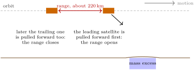
Two satellites fly one behind the other round the Earth, at an altitude of more than 500km and about 220km apart, and measure the distance between them all the time, to within a micrometre.
When they pass over a place where mass is concentrated, the leading satellite is pulled ahead first and the gap opens; then the trailing one is pulled in turn and the gap closes. From those tiny changes, month after month since 2002, the Earth’s gravity field has been mapped as it changes: the water stored in river basins rises and falls with the seasons, and the great ice sheets of Greenland and Antarctica lose mass year after year. Gravity weighs what the eye cannot see. This chapter builds the gravity field of a rotating planet from its potential, finds in it the flattening and the moment of inertia, follows its anomalies up to orbit, and then turns to one of the things gravity reveals at the surface: the bending of the lithosphere under the weight of a volcano.
You already know
Newton’s law of gravitation, the gravitational potential energy and the centrifugal force in a rotating frame are the physics books’; the moments of inertia of a solid and the Legendre polynomials P2(x)=(3x2−1)/2 are in the physics and mathematics books’ university volumes, Young’s modulus E and Poisson’s ratio ν in the physics books’ Year 3 volume. Geodesy and the flattening f=(a−b)/a of an ellipsoid of semi-axes a>b were met in grade 10. Isostasy, Airy compensation, normal gravity, the geoid, the geoid height and the gravity anomalies were defined in the Year 1 volume, in its chapter on isostasy and gravity anomalies.
3.1 The geopotential
On a rotating planet a body at rest feels the attraction of the planet’s mass and, in the frame that turns with it, the centrifugal force. Both derive from a potential.
Definition 3.1(Geopotential)
The geopotential is the potential energy per unit mass, in the frame rotating with the Earth at the angular velocity ω, of gravitation and the centrifugal force together:
where s is the distance from the rotation axis. Gravity is g=−∇W, and the surfaces W=const are its level surfaces: gravity is everywhere normal to them.
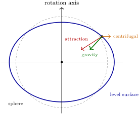
A plumb line hangs along −∇W, and still water settles on a level surface. A rotating fluid planet therefore takes the shape of one of its own level surfaces: the centrifugal potential, deepest at the equator, swells the equator and flattens the poles.
A level surface of a rotating planet (schematic, the flattening greatly exaggerated). At each point, gravity, the sum of the attraction and the centrifugal force, is normal to the level surface; it does not point at the centre, except at the poles and on the equator.
Outside the planet the gravitational potential obeys Laplace’s equation, and its solutions regular at infinity are the solid spherical harmonics.
Proposition 3.2(Spherical-harmonic expansion of the geopotential)
Outside a body of mass M and equatorial radius a, with the origin at its centre of mass and the z axis along its axis of rotation, the gravitational potential at the distance r, colatitude θ and longitude λ is
with the Legendre polynomials Pn and the associated functions Pnm; the coefficients Jn, Cnm, Snm are numbers, fitted to observations. For a body symmetric about its axis, only the zonal terms Jn remain. No term of degree 1 appears.
Proof. The separation of variables of Laplace’s equation in spherical coordinates gives the regular-at-infinity solutions r−(n+1)Pnm(cosθ)e±imλ (the mathematics books’ university volumes); any potential outside the masses is a sum of them. The term of degree 0 is −GM/r, the potential of the whole mass. The degree-1 terms are proportional to the first moments ∫r′dm′, which vanish when the origin is the centre of mass. Axial symmetry removes every term that depends on λ. ∎
Definition 3.3(Dynamical form factor)
The dynamical form factorJ2 of a planet is the coefficient of its degree-2 zonal harmonic: the largest departure of its external potential from that of a sphere, caused by its oblateness. For the Earth, J2=1.08263×10⁻³.
Theorem 3.4(MacCullagh’s formula)
Let A, B, C be the principal moments of inertia of a body of mass M about axes through its centre of mass, and I its moment of inertia about the line from the centre of mass to an external point at the distance r. To order r−3 the gravitational potential at that point is given by MacCullagh’s formula
V=−rGM−2r3G(A+B+C−3I).
For a body symmetric about the z axis (A=B), V=−rGM+r3G(C−A)P2(cosθ), so that
J2=Ma2C−A.
Proof. With r^ the unit vector towards the point and r′≪r,
∣r−r′∣1=r1+r2r^⋅r′+2r33(r^⋅r′)2−r′2+O(r−4).
Integrated over the mass, the first term gives M/r and the second vanishes (centre of mass). For the third, ∫r′2dm′=(A+B+C)/2, since A+B+C=∫2r′2dm′, and ∫(r^⋅r′)2dm′=∫r′2dm′−I, the square of the distance to the line being r′2−(r^⋅r′)2. The bracket integrates to 3(A+B+C)/2−3I−(A+B+C)/2=A+B+C−3I. For A=B, the moment about a line at colatitude θ is I=Asin2θ+Ccos2θ, and 2A+C−3I=(C−A)(1−3cos2θ)=−2(C−A)P2(cosθ). Comparing with Proposition 3.2 gives J2Ma2=C−A. ∎
The degree-2 term of the potential therefore measures the difference of the moments of inertia, not the moments themselves. The precession of the Earth’s axis, driven by the torques of the Sun and Moon on the equatorial bulge, measures the dynamical ellipticity H=(C−A)/C; together, J2 and H give C/(Ma2), the moment-of-inertia factor, 0.3308 for the Earth,
well below the 0.4 of a uniform sphere: the mass is concentrated towards the centre.
3.2 The rotating ellipsoid
Definition 3.5(Reference ellipsoid)
A reference ellipsoid is an ellipsoid of revolution, of equatorial semi-axis a and flattening f, chosen so that it is itself a level surface of a model potential: the potential of a rotating body of mass M with the angular velocity ω and the dynamical form factorJ2 of the Earth. Four constants define it; the Geodetic Reference System 1980 takes
and derives from them the flattening f=0.00335281068 (1/f=298.257222) and the semi-minor axis b=6356752.3141m.
The potential of the model, the normal potential, is known in closed form, and so is its gravity on the ellipsoid, the normal gravity of the Year 1 volume.
Proposition 3.6(Somigliana’s formula)
On a reference ellipsoid with semi-axes a, b and normal gravity γe at the equator and γp at the poles, normal gravity at the geodetic latitude φ is given by Somigliana’s formula
γ(φ)=a2cos2φ+b2sin2φaγecos2φ+bγpsin2φ.
For the Geodetic Reference System 1980, γe=9.7803267715ms−2 and γp=9.8321863685ms−2, and the series γ=9.780327(1+0.0053024sin2φ−0.0000058sin22φ)ms−2 reproduces the formula to 0.1mGal.
Proof.Admitted at this level.∎
How flat should a rotating planet be? If it is a fluid in hydrostatic equilibrium, its flattening is fixed by its rotation and by how its mass is distributed in depth.
Proposition 3.7(Clairaut and Darwin–Radau relations)
For a planet in hydrostatic equilibrium, with m=ω2a2b/(GM) the ratio of the centrifugal to the gravitational acceleration at the equator, to first order in f and m:
A uniform planet (C/Ma2=0.4) has f=5m/4; a planet whose mass is concentrated towards the centre is less flattened.
Proof.Admitted at this level.∎
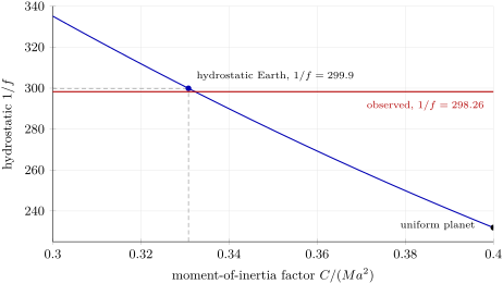
The Clairaut relation, with the Earth’s m=0.00344979, turns its measured J2 into f=0.0033488, or 1/298.6: within 0.12% of the flattening of the ellipsoid. The Darwin–Radau relation, with the moment-of-inertia factor, gives the flattening the Earth would have if it were a fluid in equilibrium: 1/299.9, against the measured 1/298.26. The Earth is a little flatter than a fluid planet with its rotation and its mass distribution would be: its equatorial bulge stands about 116m higher than hydrostatic equilibrium predicts. The Earth is not exactly a fluid in equilibrium, and the small difference is itself a measurement of the stresses its interior sustains.
The flattening of a fluid planet with the Earth’s rotation, against its moment-of-inertia factor, from the Darwin–Radau relation (computed from the Geodetic Reference System 1980). The more the mass is concentrated towards the centre, the rounder the planet. At the Earth’s 0.3308 the hydrostatic flattening is 1/299.9, a little less than the observed 1/298.26.
3.3 The geoid and the disturbing potential
The geoid is the level surface of the real geopotential that coincides with mean sea level; the reference ellipsoid is a level surface of the normal potential U with the same value, U0=W0. Their separation, the geoid height N, is set by the difference of the two potentials.
Proposition 3.8(Bruns’ formula)
Let T=W−U be the disturbing potential. The geoid height at a point is given by Bruns’ formula
N=−γT,
where T is evaluated on the geoid and γ is normal gravity there. A mass excess, which deepens the potential (T<0), raises the geoid.
Proof. Let P be on the geoid and Q the point of the ellipsoid below it, at the distance N. Since U increases outwards at the rate γ, U(P)=U(Q)+γN=U0+γN. Then W0=W(P)=U(P)+T(P)=U0+γN+T, and W0=U0 gives N=−T/γ. ∎
A geoid height of 50m is a potential difference of only 490Jkg−1, one part in 105 of the geopotential. The geoid heights of the Earth range from about +85m at Iceland to −106m in southern India,
a range of under 200m on a planet whose equatorial and polar radii differ by 21km.
3.4 Satellite gravimetry
Definition 3.9(Satellite gravimetry)
Satellite gravimetry determines the Earth’s gravity field from the motion of satellites: from the long-term perturbations of their orbits, from the changing distance between two satellites on the same orbit, or from gradiometers that measure the differences of gravity across the spacecraft.
The largest perturbation of a near-Earth orbit comes from J2. The equatorial bulge exerts a torque on the inclined orbit, which turns slowly about the Earth’s axis.
Proposition 3.10(Nodal precession)
To first order in J2, the line of nodes of a circular orbit of radius r and inclination i turns at the rate
Ω˙=−23nJ2(ra)2cosi,n=GM/r3,
westward for a prograde orbit (i<90∘), eastward for a retrograde one.
Proof. Over many revolutions the satellite acts like a ring of mass ms spread along its orbit. The degree-2 part of the potential, (GMJ2a2/r3)P2(cosθ) per unit mass, averaged over a circle inclined at i, involves ⟨cos2θ⟩=21sin2i, so ⟨P2⟩=43sin2i−21, and the ring’s energy is E(i)=ms(GMJ2a2/r3)(43sin2i−21). The torque about the line of nodes is τ=−dE/di=−23ms(GMJ2a2/r3)sinicosi. It is perpendicular to the ring’s angular momentum L=msnr2, so it turns L about the polar axis without changing its length: LsiniΩ˙=τ. With GM=n2r3, Ω˙=−23nJ2(a/r)2cosi. ∎
The rate is several degrees per day for a low orbit near the equator; at an inclination a little beyond 90∘ it matches the Sun’s yearly motion, and the orbit keeps the same orientation to the Sun all year (exercise 12). Measured on many satellites at different inclinations, such precessions give J2 and the higher zonal harmonics.
A pair of satellites does better: the changing distance between them measures the difference of the gravity they feel along the orbit. The GRACE pair flew from 2002 to 2017, and its successor, GRACE Follow-On, since its launch on 22 May 2018, its microwave link measuring the distance to within a micrometre and a laser link testing a precision up to twenty times better.
The field changes from month to month because water moves: snow and soil moisture, groundwater, lakes, the oceans, the ice sheets.
The principle of the satellite pair (schematic, not to scale). Approaching a mass excess, the leading satellite feels its attraction first and is accelerated forward, so the range between the two increases; when the trailing satellite comes over the mass the range decreases again. The range rate, measured continuously, is inverted for the gravity field.
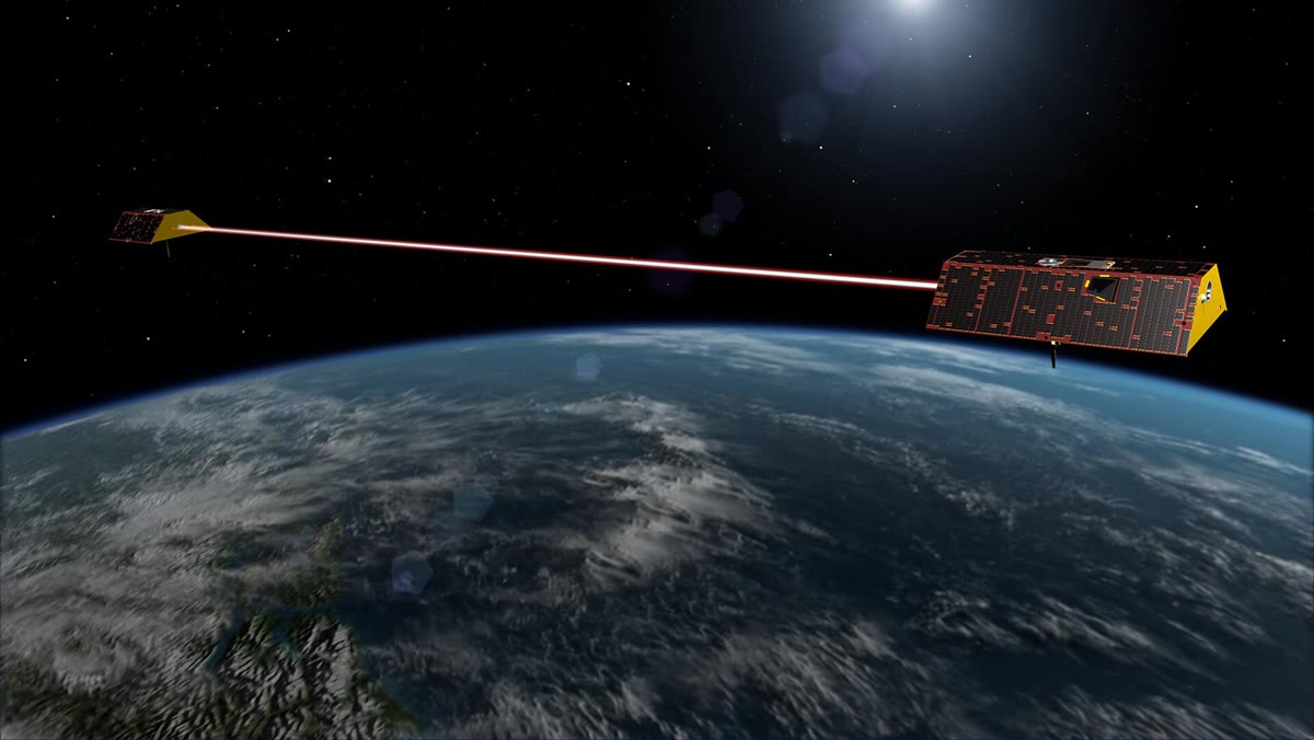
The two GRACE Follow-On satellites, an artist’s view (the distance between them is greatly shortened). The red beam stands for the laser ranging link. NASA/JPL-Caltech, public domain.
Definition 3.11(Equivalent water height)
A change of the gravity field that varies slowly over distances much larger than the thickness of the layer where the mass moved can be represented by a change of surface density σ (kgm−2) on a thin shell at the Earth’s surface. The equivalent water height is the thickness of fresh water with the same surface density:
hw=ρwσ.
A metre of water over a basin of 1×10⁶km2 is 1×10¹⁵kg, or 1000Gt. Sea level is the other side of the ledger: 360Gt of ice added to the ocean raises it by about a millimetre.
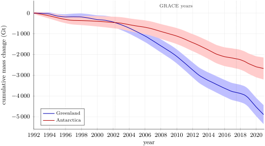
Satellite gravimetry, satellite altimetry and the balance of snowfall against ice discharge each measure the mass balance of the ice sheets; reconciled, they give the series below.
Cumulative mass change of the Greenland and Antarctic ice sheets since 1992, with one-standard-deviation bands (IMBIE 2021 reconciled estimates from altimetry, gravimetry and the input–output method). By the end of 2020 Greenland had lost 4890±460Gt and Antarctica 2670±530Gt; straight-line fits give −176Gtyr−1 and −91Gtyr−1 over 1992–2020, and −246Gtyr−1 and −127Gtyr−1 over the GRACE years.
A gravity anomaly measured at the surface is a sum of harmonics; at the altitude of a satellite, each is weakened by a factor that depends on its wavelength.
Proposition 3.12(Upward continuation)
Above the masses that cause it, a gravity anomaly that varies along the surface as Δg0coskx, with k=2π/λ, is at the height z (its upward continuation)
Δg(x,z)=Δg0e−kzcoskx.
Proof. Above the masses the anomalous potential, and with it the anomaly, satisfies Laplace’s equation ∂x2Δg+∂z2Δg=0. Separating variables, Δg=Z(z)coskx with Z′′=k2Z, whose solution bounded as z→∞ is Z=Δg0e−kz. ∎
At 400km altitude an anomaly 1000km long keeps 8% of its amplitude, one 100km long about 1×10⁻¹¹ of it: satellites see the long wavelengths, and surveys at the surface the short ones.
3.5 Flexure of the lithosphere
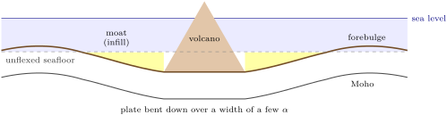
The Year 1 volume compensated a load locally, each column floating on its own. A volcano on an oceanic plate is not compensated beneath itself alone: the plate bends under it over a width of hundreds of kilometres, and the seafloor around the volcano sinks into a moat, beyond which it rises in a low arch.
Lithospheric flexure is the bending of the lithosphere under a load, modelled as the bending of a thin elastic plate floating on a fluid mantle. The plate’s resistance to bending is its flexural rigidity
D=12(1−ν2)ETe3,
and the thickness Te of the uniform elastic plate that bends like the real lithosphere is its effective elastic thickness.
Theorem 3.14(Flexure of a thin plate)
A thin elastic plate of rigidity D, bent along one direction by a load q(x) per unit area, deflected downward by w(x) and floating on a mantle of density ρm, the hollow being filled with material of density ρi, obeys the flexure equation
Ddx4d4w+(ρm−ρi)gw=q(x).
Proof. In a bent plate, the fibres above the mid-plane are shortened and those below stretched, in proportion to the curvature w′′; integrating the bending stress over the thickness gives the bending moment M=−Dw′′, with the rigidity of the definition (the plate cannot expand sideways, hence the factor 1−ν2; the physics books’ Year 3 volume). A slice dx of the plate carries the shear force V on its faces and the moment M. Vertical balance: the load qdx downward and the buoyancy of the displaced mantle (ρm−ρi)gwdx upward give dV/dx=−q+(ρm−ρi)gw. Balance of moments gives dM/dx=V. Then −Dw′′′′=M′′=V′=−q+(ρm−ρi)gw. ∎
Definition 3.15(Flexural parameter, forebulge)
The flexural parameter of a plate is the length
α=((ρm−ρi)g4D)1/4,
which sets the horizontal scale of its flexure. The forebulge is the low arch of upward flexure that a bent plate raises beyond the moat or basin next to its load.
Proposition 3.16(Line load on a continuous plate)
A line load V0 per unit length along x=0 deflects the plate by
w(x)=w0e−∣x∣/α(cosα∣x∣+sinα∣x∣),w0=8DV0α3.
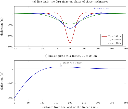
The deflection vanishes at ∣x∣=3πα/4, the edge of the moat; the forebulge crest is at ∣x∣=πα, with the height w0e−π=0.0432w0. The buoyancy of the whole deflection balances the load: ∫(ρm−ρi)gwdx=V0.
Proof. For x>0 the equation is w′′′′+4w/α4=0; the roots of r4=−4/α4 are (±1±i)/α, and the solutions that vanish far away are e−x/α(Acos(x/α)+Bsin(x/α)). Symmetry imposes w′(0)=0, which gives A=B=w0. Integrating the vertical balance across the load, the shear force V=−Dw′′′ jumps by −V0; by symmetry w′′′(0−)=−w′′′(0+), and w′′′(0+)=4w0/α3, so 8Dw0/α3=V0. The deflection vanishes where tan(x/α)=−1, first at x=3πα/4; its derivative, −(2w0/α)e−x/αsin(x/α), vanishes next at x=πα. Finally ∫0∞e−u(cosu+sinu)du=1, so ∫wdx=2w0α=V0α4/(4D)=V0/((ρm−ρi)g). ∎
Proposition 3.17(Broken plate)
A plate broken at x=0 and pushed down at its free end, as at a deep-sea trench, deflects as w=w0e−x/αcos(x/α) for x≥0: the deflection vanishes at x=πα/2, and the crest of the forebulge, the outer rise, is at x=3πα/4, with the height w0e−3π/4/2=0.067w0.
Proof. The same decaying solutions, now with the free end carrying no moment, w′′(0)=0, which gives B=0. The zero is at cos(x/α)=0; the derivative −(w0/α)e−x/α(cos+sin)(x/α) vanishes at x=3πα/4, where w=w0e−3π/4cos(3π/4). ∎
Distances are thus the key to the strength of the plate: measure where the moat ends or where the bulge crests, and α follows, then D, then Te. Since Te enters as α4/3, a fair estimate of a distance gives a good one of the thickness.
Flexure of an elastic plate (computed; E=100GPa, ν=0.25, mantle 3300kgm−3, water in the moat; vertical scale greatly exaggerated). (a) Under the load of a volcanic ridge (4.17×10¹²Nm−1), a thin plate sinks deeply and narrowly, a thick one shallowly and widely; the forebulge moves out from 112km to 316km. (b) A plate broken at a trench and pushed down by 1km: the outer rise stands 67m high, 167km from the trench.
Definition 3.18(Regional isostatic compensation)
Regional isostatic compensation is the support of a load by the buoyancy of a deflection spread over a region wider than the load, through the bending strength of the lithosphere; in Airy or Pratt compensation, by contrast, each column is compensated beneath itself.
Local and regional compensation balance the same total mass, but distribute it differently: under a narrow load on a stiff plate the root is shallow and wide, and the gravity anomaly over the load is strongly positive, flanked by negative anomalies over the moat. Around the islands of the Hawaiian Ridge, gravity and seismic profiles give effective elastic thicknesses of 17 to 37km, and 10 to 20km along the older seamounts of the Emperor chain, a difference expected from the ages of the volcanoes and of the plate they loaded; the values follow the depth of an isotherm near 350∘C in the cooling oceanic plate.
The same bending, under the weight of a mountain belt, opens the foreland basins of the Year 2 volume, in its chapter on the Alpine orogen.
A volcanic island on an oceanic plate (schematic cross-section, vertical scale exaggerated). The plate bends under the volcano; the hollow around it, the moat, fills with volcanic debris and sediment, and beyond it the plate rises in a low forebulge.
In the field— A relative gravity survey
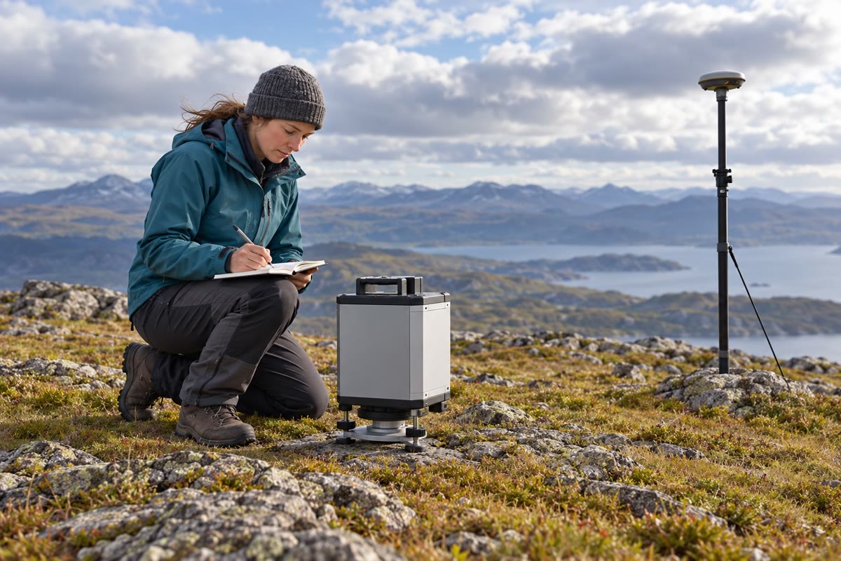
A field gravimeter on its levelling base, with a satellite antenna in the background (AI-generated illustration).
An absolute gravimeter drops a corner-cube mirror in a vacuum chamber, again and again, and times its fall with a laser interferometer and an atomic clock; it gives gravity at one station, but it is heavy and slow to set up. The survey itself is done with a relative gravimeter, a small spring balance that measures differences of gravity. The geophysicist levels it on a base plate at each station of a line, reads it, notes the time and the height, and moves on; every few hours the loop returns to a base station, so that the slow drift of the spring and the tides of the solid Earth can be measured and removed. A satellite receiver on a pole nearby gives the position and the height, because gravity changes by about 0.3mGal for every metre of height.
3.6 Exercises
Exercise 3.1★
From the Geodetic Reference System 1980 values a=6378137m and f=0.00335281068, compute the semi-minor axis b and a−b. With J2=1.08263×10⁻³ and m=0.00344979, compute the flattening that the Clairaut relation predicts, and compare.
Solution
Solution of Exercise 3.1.
b=a(1−f)=6378137×0.99664719=6356752.3m, and a−b=21384.7m, about 21.4km. Clairaut: f=(3J2+m)/2=(0.00324789+0.00344979)/2=0.0033488, or 1/298.61, against 1/298.26: 0.12% smaller, the size of the second-order terms the relation neglects.
Exercise 3.2★
In a dry year, a river basin of 5.0×10⁵km2 loses 60Gt of water. Compute the change of equivalent water height. By how much would the same mass raise sea level, taking 360Gt per millimetre?
Solution
Solution of Exercise 3.2.
σ=6.0×10¹³kg/5.0×1011m2=120kgm−2, so hw=120/1000=0.12m: 12cm of water. Delivered to the ocean, 60/360=0.17mm of sea level.
Exercise 3.3★
With the series γ=9.780327(1+0.0053024sin2φ−0.0000058sin22φ)ms−2, compute normal gravity at the equator, at 45∘ and at the poles. Express the difference between the pole and the equator in milligals.
Solution
Solution of Exercise 3.3.
At the equator γ=9.780327ms−2. At 45∘, sin2φ=0.5 and sin22φ=1: γ=9.780327×1.0026454=9.806200ms−2. At the poles, 9.780327×1.0053024=9.832186ms−2. The difference is 0.051859ms−2, or 5186mGal.
Exercise 3.4★
Compute the flexural rigidity and the flexural parameter of oceanic plates with Te=10km and Te=30km (E=100GPa, ν=0.25, ρm−ρw=2270kgm−3, g=9.81ms−2). Where are the edge of the moat and the forebulge under a line load?
Solution
Solution of Exercise 3.4.
D=ETe3/(12(1−ν2))=1011Te3/11.25: 8.89×10²¹Nm for 10km, 2.40×10²³Nm for 30km. With (ρm−ρw)g=22269Nm−3, α=(4D/22269)1/4: 35.5km and 81.0km. The moat ends at 3πα/4, 84km and 191km; the forebulge crests at πα, 112km and 255km.
Exercise 3.5★★
(a) A geoid height of +50m: compute the disturbing potential there, taking γ=9.80ms−2. (b) Over 100km the geoid rises by 10m. By what angle does the plumb line there differ from the normal to the ellipsoid? Give it in seconds of arc.
Solution
Solution of Exercise 3.5.
(a) T=−γN=−9.80×50=−490Jkg−1. (b) The geoid tilts by 10/100000=1.0×10−4 rad relative to the ellipsoid, and the plumb line, normal to the geoid, by the same angle relative to the ellipsoid’s normal: 1.0×10−4×206265=20.6′′.
Exercise 3.6★★
From J2=1.08263×10⁻³ and the moment-of-inertia factor C/(Ma2)=0.3308, compute the dynamical ellipticity H=(C−A)/C and 1/H. Which of the two numbers would a uniform Earth with the same J2 change?
Solution
Solution of Exercise 3.6.
H=J2/(C/Ma2)=1.08263×10−3/0.3308=0.0032728, and 1/H=305.55. J2 is the same by hypothesis; a uniform Earth would have C/(Ma2)=0.4 and so H=J2/0.4=0.0027066: precession would be slower. Measuring both J2 and H is what reveals the concentration of mass towards the centre.
Exercise 3.7★★
A satellite flies a circular orbit 500km above the equatorial radius (a=6378.137km, GM=3.986005×10¹⁴m3s−2), inclined at 89∘. Compute its period and the rate of nodal precession in degrees per day. Why do gravity missions choose near-polar orbits?
Solution
Solution of Exercise 3.7.
r=6878.137km; n=GM/r3=1.10678×10−3rads−1, a period of 2π/n=94.6min. Ω˙=−1.5×1.10678×10−3×1.08263×10−3×(6378.137/6878.137)2×cos89∘=−2.70×10−8rads−1, or −0.134∘ per day, westward. A near-polar orbit passes over every latitude, so the whole Earth is mapped; it also precesses slowly, so that the ground tracks fill in regularly.
Exercise 3.8★★
Two anomalies of 10mGal at the surface have wavelengths of 100km and 1000km. Compute their amplitudes at 500km altitude.
Seaward of a trench, the crest of the outer rise lies 120km from the trench axis. Taking the broken-plate model with water above the plate, compute α, D and Te, and the distance where the plate crosses its unflexed level.
Solution
Solution of Exercise 3.9.
3πα/4=120km gives α=50.9km. D=(ρm−ρw)gα4/4=22269×(50930)4/4=3.75×1022Nm, and Te=(11.25D/E)1/3=16.2km. The plate crosses its unflexed level at πα/2=80km from the trench.
Exercise 3.10★★★
(a) Check that w=w0e−u(cosu+sinu), u=x/α, satisfies Dw′′′′+(ρm−ρi)gw=0 for x>0, with α as defined. (b) Show that the bending moment −Dw′′ is greatest under the load and changes sign at x=πα/4. (c) Where is the plate most likely to crack at its upper surface, and why?
Solution
Solution of Exercise 3.10.
(a) With u=x/α, d4/dx4=α−4d4/du4. Writing cosu+sinu=2cos(u−π/4), the function is 2w0Ree(−1+i)u−iπ/4, and (−1+i)4=−4: so w′′′′=−4w/α4. Then Dw′′′′+(ρm−ρi)gw=(−4D/α4+(ρm−ρi)g)w=0, since α4=4D/((ρm−ρi)g). (b) w′′=−(2w0/α2)e−u(cosu−sinu), so M=−Dw′′=(2Dw0/α2)e−u(cosu−sinu): largest in magnitude at u=0, zero where tanu=1, x=πα/4. (c) Under the load the plate is concave upward, its upper surface in compression; beyond πα/4 it is convex upward, its upper surface stretched. There M′∝−e−ucosu vanishes at u=π/2: the stretching is greatest at x=πα/2, on the outer slope of the moat towards the forebulge, where ∣M∣ is e−π/2=21% of its value under the load. That is where normal faults and cracks would open at the top of the plate.
Exercise 3.11★★★
With m=0.00344979 and C/(Ma2)=0.3308, invert the Darwin–Radau relation for the hydrostatic flattening. Compare with f=0.00335281: compute the difference and the excess height of the equator above the hydrostatic shape. What does it say about the mantle?
Solution
Solution of Exercise 3.11.
1+η=2.5(1−1.5×0.3308)=1.2595, so 1+η=1.5863 and 25m/f=2.5863: fh=2.5×0.00344979/2.5863=0.0033346, 1/fh=299.9. The difference f−fh=1.82×10⁻⁵; times a, the equator stands 116m above the hydrostatic figure. The Earth is not quite a fluid in equilibrium: its interior sustains stresses, from the strength of the lithosphere or the flow and density differences of the mantle, that hold the shape a little away from it.
Exercise 3.12★★★
A satellite on a circular orbit 700km high is to keep the same orientation relative to the Sun all year: its node must advance by 360∘ in a tropical year of 365.242 days. Compute the inclination required.
Solution
Solution of Exercise 3.12.
The node must advance by 2π/(365.242×86400)=1.991×10−7rads−1. At r=7078.137km, n=1.0602×10⁻³rads−1 and 23nJ2(a/r)2=1.398×10−6, so cosi=−1.991×10⁻⁷/1.398×10−6=−0.1424 and i=98.2∘: a slightly retrograde, sun-synchronous orbit.
3.7 Problem: The Moat around the Oru Ridge
Problem 3.1
Weekend problem — the figure of the Earth, a volcanic load, its flexural moat and what satellites see of it
Oru is an invented volcanic ridge in an ocean: a straight chain of coalesced volcanoes 400km long, built on old oceanic lithosphere. Its cross-section is taken as a triangle 80km wide at its base and 6km high, of density 2800kgm−3, standing on a sea floor 5km deep. Mantle 3300kgm−3, sea water 1030kgm−3, E=100GPa, ν=0.25, g=9.81ms−2, G=6.674×10⁻¹¹m3kg−1s−2.
Part I — The figure of the Earth. Use the Geodetic Reference System 1980: a=6378137m, b=6356752.3m, GM=3.986005×10¹⁴m3s−2, J2=1.08263×10⁻³, ω=7.292115×10⁻⁵rads−1, f=0.00335281; and C/(Ma2)=0.3308.
Compute m=ω2a2b/(GM).
Compute the flattening that the Clairaut relation gives from J2 and m, and its inverse.
Compute the hydrostatic flattening from the Darwin–Radau relation, and its inverse.
Compare both with the observed flattening. By how many metres does the equator stand above the hydrostatic figure?
Compute the dynamical ellipticity H=(C−A)/C.
Part II — The load.
Compute the area of the ridge’s cross-section.
Compute the line load V0, taking the whole ridge as submerged, so that it weighs (ρv−ρw)g per unit volume.
If the ridge were compensated locally, in Airy fashion, by a root of its own rock in the mantle, how deep would the root be under the crest?
Under local compensation, the root would end at the foot of the ridge, 40km from its axis. Bathymetry shows a moat out to 165km. What does this tell you?
Part III — The flexural moat. The moat is filled with water (ρi=ρw). A seismic profile across the ridge finds the top of the oceanic crust back at its regional depth 165km from the axis, and the crest of the forebulge220km from the axis.
Check that the buoyancy of the whole deflection, 2w0α(ρm−ρw)g, balances V0.
Compare Te with the values found along the Hawaiian Ridge, 17 to 37km. Compare the deflection under the axis with the Airy root of question 8.
Part IV — Gravity over the moat. Take one harmonic of the flexure, of wavelength 2πα and amplitude W=500m, deflecting both the sea floor (crust 2900kgm−3 under water, 5km below sea level) and the Moho (mantle under crust, 12km below sea level). A thin sheet of surface density σ produces the anomaly 2πGσ just above it.
Compute the wavelength and the wavenumber k of the harmonic.
Compute the amplitude of the anomaly at sea level due to the deflected sea floor, continued up from 5km depth.
Compute that of the deflected Moho, and the total.
Compute the total at the altitude of a satellite, 400km above sea level.
By what factor is a harmonic of wavelength 80km, the width of the ridge, weakened at that altitude? What can the satellite resolve?
To what spherical-harmonic degree n≈2πR/λ does the harmonic of question 18 correspond (R=6371km)?
3.1+η=2.5(1−1.5×0.3308)=1.2595, 25m/fh=2+0.5863, so fh=0.0033346 and 1/fh=299.88.
4. The Clairaut value, 1/298.61, is within 0.12% of the observed 1/298.26; the hydrostatic one, 1/299.88, is smaller by Δf=1.82×10⁻⁵, and aΔf=116m: the equator stands 116m above the hydrostatic figure.
5.H=1.08263×10⁻³/0.3308=0.0032728 (1/305.6).
6.21×80km×6km=240km2=2.40×10⁸m2.
7.V0=(2800−1030)×9.81×2.40×108=4.17×10¹²Nm−1.
8. Airy: (ρm−ρv)r=(ρv−ρw)h, so r=6×1770/500=21.2km under the crest.
9. The sea floor is deflected far beyond the foot of the ridge: the load is not compensated column by column but by the bending of the plate over a region four times wider. The plate has strength: regional compensation.
10.α=165/(3π/4)=70.0km.
11.α=220/π=70.0km: the same, as a single elastic plate requires.
16.2×1334×7.00×104×2270×9.81=4.16×10¹²Nm−1, equal to V0 to within the rounding of D.
17.24.7km lies inside the range of the Hawaiian Ridge. The plate sinks 1.3km under the axis instead of growing a root of 21km: the same buoyancy is spread over the 330km of the moat.
18.λ=2π×70.0km=440km, k=1/α=1.43×10−5m−1.
19.σ=(2900−1030)×500=9.35×10⁵kgm−2, so 2πGσ=3.92×10⁻⁴ms−2=39.2mGal at the sea floor; times e−k×5km=0.931, 36.5mGal at sea level (negative where the plate is pushed down).
20.σ=(3300−2900)×500=2.0×10⁵kgm−2: 8.39mGal, times e−k×12km=0.843, 7.07mGal. The total is 43.6mGal.
21.e−k×400km=e−5.71=0.0033: 0.14mGal.
22.e−2π×400/80=e−31.4=2.3×10−14: the satellite sees nothing of the ridge itself, only the broad flexure, and even that weakened three-hundred-fold; the ridge’s own anomaly must be measured at sea.