21Ocean Dynamics

Through the Strait of Florida the Gulf Stream carries about $32\,\mathrm{Sv}$ of water northward, and it grows as it follows the coast north, to about $150\,\mathrm{Sv}$ near $40{}^{\circ}$ N. On the other side of the same ocean, off Portugal and north Africa, nothing like it flows south: the water that the Gulf Stream carries north returns towards the equator as a slow, broad drift across thousands of kilometres of open sea. Every ocean basin of the Northern Hemisphere has the same lopsided shape, its fast current on the western side. The asymmetry follows from the wind, from the friction of the sea, and from one fact about the Earth: the Coriolis parameter grows towards the pole.

You already know

The tidal force of the Moon and the Sun, spring and neap tides, are in the physics books. The wind stress, the Ekman layer, the Ekman transport and the Ekman spiral, upwelling and downwelling, the gyres, the western boundary currents, the sverdrup ($1\,\mathrm{Sv} = 10^{6}\,\mathrm{m}^{3}/\mathrm{s}$), the meridional overturning circulation and the formation of deep water are in the Year 1 volume, in its chapter on the ocean circulation; there the wind stress is written $\vec T$, here $\vec\tau$. The Coriolis parameter, the $\beta$-plane, the Rossby radius and the geostrophic balance are in Chapter 19; vorticity and potential vorticity in Chapter 20.

21.1 The Ekman layer derived

In the Year 1 volume the Ekman transport was found from a balance of forces on the whole layer, and the spiral of velocities inside it was stated. With a turbulent friction of constant eddy viscosity $A_z$, the spiral follows from the equations in a few lines. Write the horizontal velocity as a complex number, $W = u + \mathrm iv$, and the wind stress as $\tau = \tau_x + \mathrm i\tau_y$; a multiplication by $-\mathrm i$ turns a vector by $90{}^{\circ}$ clockwise, to its right seen from above.

Theorem 21.1 (Velocity profile of a steady wind-driven surface layer)

In a steady, horizontally uniform ocean of great depth and constant density $\rho$, with a constant vertical eddy viscosity $A_z$ and the Coriolis parameter $f > 0$, the current driven by a wind stress $\tau$ is

$$W(z) = W_0\,\mathrm e^{(1+\mathrm i)z/\delta},\qquad W_0 = \frac{\tau}{\rho\sqrt{fA_z}}\,\mathrm e^{-\mathrm i\pi/4},\qquad \delta = \sqrt{\frac{2A_z}{f}} ,$$

for $z \le 0$. The surface current is turned $45{}^{\circ}$ to the right of the stress; with depth it turns further right and decays as $\mathrm e^{z/\delta}$; the total transport $\int_{-\infty}^0 W\,\mathrm dz = -\mathrm i\tau/(\rho f)$ is at right angles to the right of the stress.

The theorem recovers both results of the Year 1 volume: Ekman’s surface current at $45{}^{\circ}$ and the transport $\tau/(\rho f)$, at right angles to the stress and independent of $A_z$, which is never well known. At the depth $\pi\delta$ the current flows against the surface current, reduced by $\mathrm e^{-\pi}$, to $4\,\%$.

Definition 21.2 (Ekman depth; Ekman pumping)

The Ekman depth is $D_E = \pi\delta = \pi\sqrt{2A_z/f}$, the depth at which the current of the Ekman spiral flows opposite to the surface current; it measures the thickness of the Ekman layer. Ekman pumping is the vertical velocity $w_E$ at the base of the Ekman layer forced by the convergence or divergence of the Ekman transport: downward where the transports converge, upward, sometimes called Ekman suction, where they diverge.

Proposition 21.3 (Ekman pumping)

With the vertical velocity zero at the sea surface, the Ekman pumping is

$$w_E = \operatorname{curl}_z\frac{\vec\tau}{\rho f} = \frac{1}{\rho f}\Big(\frac{\partial\tau_y}{\partial x} - \frac{\partial\tau_x}{\partial y}\Big) + \frac{\beta\tau_x}{\rho f^2} ,$$

upward positive.

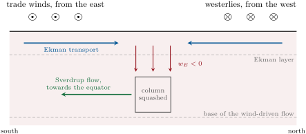
A wind that turns cyclonically over the sea, its curl positive, draws water up from below the layer; an anticyclonic wind pushes it down. Over the subtropical oceans the trade winds blow from the east on the equatorward side, the westerlies from the west on the poleward side. Their Ekman transports, north under the trades and south under the westerlies, converge between them: the surface water piles up and is pumped down, as in the figure below. Along a coast where the wind blows with the coast on its left (in the Northern Hemisphere), the transport leaves the shore and the coastal upwelling of the Year 1 volume is Ekman suction concentrated against a wall.

21.2 The Sverdrup balance

Below the Ekman layer the ocean is geostrophic. A column of water that is squashed by Ekman pumping must, to keep its potential vorticity $f/h$, move to where $f$ is smaller: towards the equator. In 1947 H. U. Sverdrup made the argument quantitative for the whole depth of the wind-driven flow.

Theorem 21.4 (Sverdrup balance)

In a steady ocean in which the non-linear terms and the lateral friction are negligible, the interior is geostrophic below the Ekman layer, and the vertical velocity vanishes at some depth $-H$, the total northward volume transport per unit width of the wind-driven flow obeys the Sverdrup balance

$$\beta V = \frac{1}{\rho}\operatorname{curl}_z\vec\tau = \frac{1}{\rho}\Big(\frac{\partial\tau_y}{\partial x} - \frac{\partial\tau_x}{\partial y}\Big) .$$

The balance is remarkable for what it does not need: neither the depth of the flow, nor its vertical structure, nor the eddy viscosity, only the curl of the wind and $\beta$. Sverdrup derived it from the equations of motion integrated down to a depth of no motion, and tested it against the hydrographic sections of the research vessels Carnegie and Bushnell in the eastern tropical Pacific, between $34{}^{\circ}$ N and $10{}^{\circ}$ S, with a depth of no motion at $1000\,\mathrm{m}$: the transports computed from the wind matched those computed from the density field, even where the currents ran against the wind. Later work with better winds found the best agreement with a depth of no motion near $500\,\mathrm{m}$, and measurements of the mean stress in the equatorial Pacific in 1999 found the flow there in Sverdrup balance. Whether the balance holds everywhere is harder to show than to assume: almost every theory of the ocean circulation starts from it.

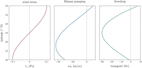
Take the invented basin of this chapter’s problem: between $20{}^{\circ}$ and $50{}^{\circ}$ N, $6000\,\mathrm{km}$ wide, under a zonal stress $\tau_x = -\tau_0\cos(\pi(\varphi - 20{}^{\circ})/30{}^{\circ})$ with $\tau_0 = 0.1\,\mathrm{Pa}$, easterly at $20{}^{\circ}$ N, westerly at $50{}^{\circ}$ N, zero at $35{}^{\circ}$ N. Over almost all the basin the stress curl is negative: the water is pumped down, by about $35\,\mathrm{m}$ a year at $35{}^{\circ}$ N, and the interior flows south, $4.9\,\mathrm{m}^{2}/\mathrm{s}$ per metre of width at $35{}^{\circ}$ N, $29.4\,\mathrm{Sv}$ across the basin. Computed from the observed winds, the Sverdrup transport of the North Atlantic subtropical gyre reaches about $30\,\mathrm{Sv}$ near $28{}^{\circ}$ N.

The Sverdrup transport fixes $V$ at every point, but a streamfunction needs a boundary condition, and a meridional wall can take only one. If the interior satisfies no flow through the eastern wall, the southward flow has nowhere to go at the western wall; the mass is returned by a current that Sverdrup’s equations, without friction, cannot describe.

21.3 Western intensification

In 1948 H. Stommel added the simplest friction to the simplest ocean, and found the return flow crowded against the western wall, as in the Year 1 volume’s figure of his gyre. He found it only with a Coriolis parameter that grows northward: with no rotation, or with a uniform one, his gyre was symmetric.

Definition 21.5 (Western intensification; Stommel model; Munk boundary layer)

Western intensification is the crowding of the return flow of a wind-driven gyre into a narrow, fast current against the western side of the basin. The Stommel model is a homogeneous ocean of constant depth in a rectangular basin, driven by a zonal wind stress and slowed by a bottom friction proportional to the depth-integrated velocity, with a rate $r$; its transport streamfunction $\psi$ ($U = -\partial\psi/\partial y$, $V = \partial\psi/\partial x$) obeys

$$r\nabla^2\psi + \beta\frac{\partial\psi}{\partial x} = \frac{1}{\rho}\operatorname{curl}_z\vec\tau ,\qquad \psi = 0 \text{ on the walls.}$$

The Munk boundary layer is the western boundary layer of the same gyre when a lateral eddy viscosity $A_H$ replaces the bottom friction; its width scale is $\delta_M = (A_H/\beta)^{1/3}$.

The equation is the Sverdrup balance with the curl of the bottom friction added: integrated over the depth, $\beta V = \rho^{-1}\operatorname{curl}_z \vec\tau - r\zeta_T$, where $\zeta_T = \nabla^2\psi$ is the vorticity of the transport.

Theorem 21.6 (Western boundary layer of the Stommel gyre)

In a basin $0 \le x \le X$, $0 \le y \le L$, with $\tau_x = -\tau_0 \cos(\pi y/L)$ and $\delta_S = r/\beta \ll X$, the Stommel streamfunction is, to leading order in $\delta_S/X$,

$$\psi = A\sin\frac{\pi y}{L}\Big[(X - x) - X\mathrm e^{-x/\delta_S}\Big], \qquad A = \frac{\pi\tau_0}{\rho\beta L} .$$

The interior carries $AX\sin(\pi y/L)$ south; a boundary layer of width $\delta_S$ against the western wall returns it north; no boundary layer can exist against the eastern wall.

The same answer comes from vorticity. Over the interior the wind gives each column negative vorticity, and the column pays for it by moving south, to smaller $f$. On the way back north it gains planetary vorticity and must lose it, which only friction can do. In a northward current whose speed falls off eastward from near the western wall, $\partial v/\partial x < 0$ over most of its width: the current’s vorticity is negative, and friction, acting against it, supplies the positive vorticity that the columns need. A northward current against an eastern wall would have positive vorticity, and friction would take away the wrong sign.

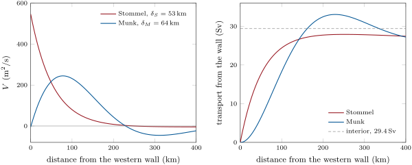
With $r = 10^{-6}\,\mathrm{s}^{-1}$ at $35{}^{\circ}$ N, $\delta_S = 53\,\mathrm{km}$, and the northward flow occupies the first $250\,\mathrm{km}$ from the wall. In 1950 W. H. Munk replaced the bottom friction by a lateral eddy viscosity $A_H$, which acts on the shear within the current; the equation gains a term $A_H\nabla^4\psi$, and near the western wall the correction becomes $\mathrm e^{-x/2\delta_M}$ times an oscillation, $\cos(\sqrt3x/2\delta_M)$ and $\sin(\sqrt3x/2\delta_M)$. With $A_H = 5 \times 10^{3}\,\mathrm{m}^{2}/\mathrm{s}$ the northward jet is about $225\,\mathrm{km}$ wide ($233\,\mathrm{km}$ in the basin of the figure), with a weak countercurrent beyond it, a shape close to the Gulf Stream and the Kuroshio. As in Stommel’s layer, the transport of the jet does not depend on the friction but only on the wind-stress curl, the width of the basin and $\beta$. From the winds of his time Munk computed $36\,\mathrm{Sv}$ for the Gulf Stream and $39\,\mathrm{Sv}$ for the Kuroshio, about half the transports then measured; with a better drag coefficient and finer averages of the stress, $32\,\mathrm{Sv}$ was found for the Gulf Stream in 1978. Measured mainly with a submarine cable, the Gulf Stream in the Strait of Florida has carried $31.7\,\mathrm{Sv}$ on average since 2004. Downstream it grows to about $150\,\mathrm{Sv}$ near $40{}^{\circ}$ N, and offshore of Cape Hatteras a strong recirculation, which the linear theory does not contain, spoils the agreement.

21.4 The abyssal circulation

The deep ocean is filled from a few places. In the Year 1 volume, deep water forms where surface water is cooled and made dense in the far North Atlantic and round Antarctica, and spreads through the basins as North Atlantic Deep Water and Antarctic Bottom Water. Between 1958 and 1960 H. Stommel, A. B. Arons and A. J. Faller asked how it spreads, using the same vorticity argument as Sverdrup.

Definition 21.7 (Stommel–Arons model)

The Stommel–Arons model of the abyssal circulation supposes that deep water is supplied by convection at a few high-latitude sources, that it returns to the upper ocean by a slow, uniform upwelling $W_0$ through the base of the thermocline, balanced by downward mixing of heat, and that the interior flow is geostrophic and conserves potential vorticity. The circulation is closed by deep western boundary currents.

Proposition 21.8 (Poleward interior flow of the abyss)

In the Stommel–Arons model, over a flat bottom, the depth-integrated northward transport of the abyssal interior is

$$V = \frac{f}{\beta}W_0 = a\tan\varphi\,W_0 ,$$

poleward in both hemispheres when $W_0 > 0$.

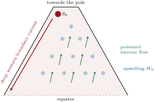
The result is counter-intuitive: the abyssal interior flows towards the sources, not away from them. Stommel and Arons built rotating-tank experiments to convince themselves. The water from the sources travels along the western walls, in deep western boundary currents that feed the interior as they go. In a sector of ocean between the equator and the pole with the whole source $S_0$ near the pole, the western boundary current carries $2S_0\sin\varphi$ towards the equator, twice the source at the pole and nothing at the equator: the excess over $S_0$ is water recirculating from the interior. The model makes the deep circulation driven by mixing, not by sinking: without the upwelling, convection would only fill the abyss with a stagnant pool of cold water. Its transit times range from a few centuries near the sources to nearly a thousand years in the North Pacific. Over the real ocean floor the ridges divide the basins, mixing is strong over rough topography, and the deep flow is far more zonal than the model’s. Its lasting prediction is the deep western boundary current: in the North Atlantic one returns about $14\,\mathrm{Sv}$ of water at $2\,{}^{\circ}\mathrm{C}$ to the south, while the Gulf Stream carries the warm water north.

The interior of the model, like Sverdrup’s, is geostrophic, and the geostrophic currents of the deep sea are measured in the way that Sverdrup measured his: from the density.

Definition 21.9 (Dynamic method)

The dynamic method computes the geostrophic current between two hydrographic stations from the density measured at both, relative to a reference pressure level where the current is taken to be zero or known. The geopotential distance between two pressure surfaces, $\int\alpha\,\mathrm dp$ with $\alpha = 1/\rho$ the specific volume, is split into a standard part, the same at both stations, and the geopotential anomaly $\Delta\Phi$; the current at the upper surface, at right angles to the line between stations $A$ and $B$, a distance $L$ apart, is

$$v = \frac{\Delta\Phi_B - \Delta\Phi_A}{fL} .$$

Why not measure the pressure directly, as meteorologists do? A geostrophic current of $10\,\mathrm{cm}/\mathrm{s}$ at $30{}^{\circ}$ needs a pressure gradient of $7.5 \times 10^{-3}\,\mathrm{Pa}/\mathrm{m}$, $750\,\mathrm{Pa}$ across $100\,\mathrm{km}$: the weight of $7.4\,\mathrm{cm}$ of sea water. No pressure gauge on the sea floor can be levelled that well. The density, computed to a few parts per million, gives instead the slope of one pressure surface relative to another. The lighter, warmer water lies to the right of the current, looking downstream, in the Northern Hemisphere. Across the Gulf Stream the surfaces of constant density change depth by more than a kilometre over $100\,\mathrm{km}$.

Method 21.10 (Geostrophic current from two stations)

1. At each station, compute the specific-volume anomaly $\delta = \alpha(S, T, p) - \alpha(35, 0, p)$ from the measured salinity, temperature and pressure.
2. Integrate it from the reference pressure up to each pressure $p$: $\Delta\Phi(p) = \int_p^{p_{\text{ref}}}\delta\,\mathrm dp$.
3. At each pressure, $v(p) = (\Delta\Phi_B - \Delta\Phi_A)/(fL)$ is the current relative to the reference level, positive with station $B$ on the right.
4. Add the current at the reference level if it is known, from a float drifting there or from the sea-surface slope measured by satellite.

In the field — An array of floats

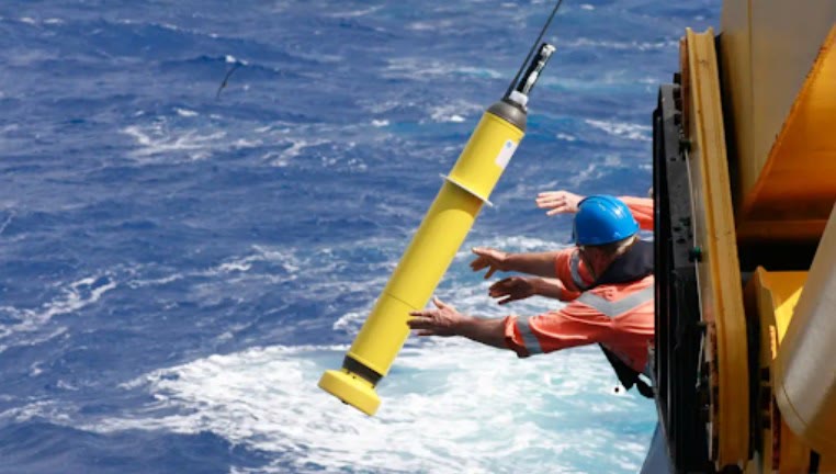
Figures as of 2024

Close to four thousand Argo floats drift through the world ocean. Lowered over the side of a ship, a float sinks to about $1000\,\mathrm{m}$ and drifts there for about nine days; it then sinks to $2000\,\mathrm{m}$ and rises to the surface, measuring conductivity, temperature and pressure on the way, and the cycle starts again about every ten days; Deep Argo floats profile to $6000\,\mathrm{m}$. In July 2024 the array collected its three millionth profile. From the profiles oceanographers compute the geopotential anomalies of the dynamic method at every float, and the float’s own displacement between two surfacings gives the mean current at its parking depth: the reference velocity that Sverdrup had to assume is now measured.

21.5 Ocean tides

Twice a day, a little less than an hour later each day, the sea rises and falls. The physics books explain the tidal force: the Moon’s attraction is stronger on the near side of the Earth than at its centre, and weaker on the far side, so that relative to the centre the water is pulled out along the line to the Moon on both sides.

Definition 21.11 (Equilibrium tide; tidal constituent)

The equilibrium tide is the shape that the surface of an ocean covering the whole Earth would take if it followed the tide-generating potential instantly, without inertia. A tidal constituent is one of the harmonic terms, each with a fixed frequency set by the motions of the Moon and the Sun and an amplitude and phase found at each place, whose sum makes the tide; they are named by a letter and the number of cycles per day, such as M$_2$, the principal lunar semi-diurnal constituent.

Theorem 21.12 (Equilibrium tide of the Moon)

For the Moon, of mass $M$ at distance $d$ from the centre of the Earth, of mass $M_E$ and radius $a$, the equilibrium tide at an angle $\theta$ from the point under the Moon is

$$\eta = K\,\frac{3\cos^2\theta - 1}{2},\qquad K = \frac{M}{M_E}\Big(\frac{a}{d}\Big)^3 a .$$

With the mass ratio $0.0123$, $d = 384\,400\,\mathrm{km}$ and $a = 6371\,\mathrm{km}$, $K = 0.357\,\mathrm{m}$: the sea stands $0.36\,\mathrm{m}$ high under the Moon and on the opposite side, and $0.18\,\mathrm{m}$ low on the great circle between, a range of $0.54\,\mathrm{m}$. At latitude $\varphi$, with the Moon at declination $\delta$ and at hour angle $H$, $\cos\theta = \sin\varphi\sin\delta + \cos\varphi\cos\delta\cos H$. As the Earth turns under the two bulges a place passes through two high waters a lunar day, $24\,\mathrm{h}$ $50\,\mathrm{min}$: the semi-diurnal tide. When the Moon stands north or south of the equator the two bulges are tilted, and the two high waters of a day are unequal, as the figure below shows. The Sun raises a tide of the same form, $0.46$ times as large; the two add at new and full moon, at spring tides, and partly cancel at the quarters.

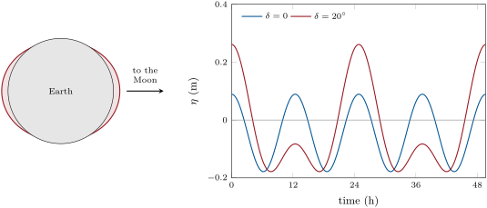
The harmonic analysis of the equilibrium tide gives its constituents. The five largest, with their equilibrium amplitudes, are in the table below. At least 39 constituents are needed to predict a port’s tide to a thousandth of its largest term, and a gauge must run for more than 18.6 years, the period of the modulation of the lunar tides, to separate them all.

The real tide is not the equilibrium tide. To keep a bulge under the Moon on the equator, the tide would have to travel round the Earth in a lunar day, at about $460\,\mathrm{m}/\mathrm{s}$, a speed that a long gravity wave reaches only in an ocean $22\,\mathrm{km}$ deep; and the continents stop it. The tide is instead a forced long wave, sloshing in each basin near resonance, and the rotation of the Earth makes it turn round the basin.

Definition 21.13 (Kelvin wave)

An oceanic Kelvin wave is a long gravity wave that travels along a coast, or along the equator, with no velocity across it, its height decreasing exponentially away from the coast over the Rossby radius. Along a coast it travels with the coast on its right in the Northern Hemisphere, on its left in the Southern.

Theorem 21.14 (Coastal Kelvin wave)

In an ocean of uniform depth $H$ on an $f$-plane, with $f > 0$, bounded by a straight coast along $y = 0$ and lying in $y > 0$, the linear shallow-water equations have the solutions with $v = 0$

$$\eta = \mathrm e^{-y/L_R}F(x - ct),\qquad u = \frac{g}{c}\,\eta,\qquad c = \sqrt{gH},\quad L_R = \frac{c}{f},$$

for any profile $F$, and no solution with $v = 0$ travels in the direction $-x$.

Over the deep ocean, $4000\,\mathrm{m}$ deep, $c = 198\,\mathrm{m}/\mathrm{s}$ and the Rossby radius is about $2000\,\mathrm{km}$ at mid-latitudes: the tide sweeps round a whole basin. Over a shelf sea $50\,\mathrm{m}$ deep, $c = 22\,\mathrm{m}/\mathrm{s}$, the Rossby radius is under $200\,\mathrm{km}$, and an M$_2$ wavelength is about $1000\,\mathrm{km}$. In a gulf, the tide entering along one coast as a Kelvin wave returns along the opposite coast, again with the coast on its right; the two waves cancel at points in between.

Definition 21.15 (Amphidromic point; cotidal line; co-range line)

An amphidromic point is a point where the amplitude of a tidal constituent is zero and round which its high water turns. A cotidal line joins the places where a constituent’s high water comes at the same time; a co-range line joins the places of equal tidal range. Cotidal lines radiate from the amphidromic points; co-range lines circle them.

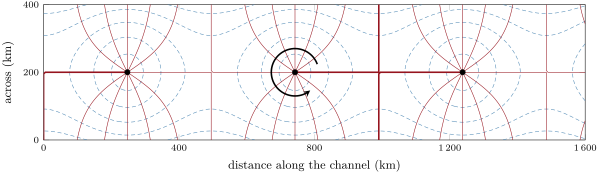
The maps of the ocean tide made from satellite altimetry, accurate to about $2\,\mathrm{cm}$ in the deep sea, show this structure everywhere: the M$_2$ crest turns anticlockwise round the amphidromes of the Northern Hemisphere basins and clockwise in the Southern, and the largest ranges are on the coasts. The tides dissipate $3.75\,\mathrm{TW}$, $3.5\,\mathrm{TW}$ of it in the ocean, about two thirds of the M$_2$ energy on the shelves and in shallow seas and one third through internal waves in the deep ocean. That energy lengthens the day by about $2.07\,\mathrm{ms}$ a century and pushes the Moon away by $3.86\,\mathrm{cm}$ a year; and the part lost in the deep ocean mixes it, supplying some of the mixing that, in the Stommel–Arons picture, drives the abyssal circulation.

21.6 Exercises

Exercise 21.1 ★

A westerly wind stress of $0.12\,\mathrm{Pa}$ blows over the sea at $40{}^{\circ}$ N ($\rho = 1025\,\mathrm{kg}/\mathrm{m}^{3}$, $\Omega = 7.292\,115 \times 10^{-5}\,\mathrm{rad}/\mathrm{s}$). Compute the Ekman volume transport per metre of width and its direction, and the transport across a section $1000\,\mathrm{km}$ long, in sverdrups.

Solution

Solution of Exercise 21.1.

$f = 9.37 \times 10^{-5}\,\mathrm{s}^{-1}$; $\tau/(\rho f) = 0.12/(1025\times9.37 \times 10^{-5}) = 1.25\,\mathrm{m}^{2}/\mathrm{s}$, to the right of the wind: south. Across $1000\,\mathrm{km}$, $1.25 \times 10^{6}\,\mathrm{m}^{3}/\mathrm{s}$, $1.25\,\mathrm{Sv}$.

Exercise 21.2 ★

With $A_z = 0.05\,\mathrm{m}^{2}/\mathrm{s}$, compute the Ekman depth at $45{}^{\circ}$ N. What fraction of the surface current remains at that depth?

Solution

Solution of Exercise 21.2.

$f = 1.031 \times 10^{-4}\,\mathrm{s}^{-1}$; $D_E = \pi\sqrt{2\times0.05/1.031 \times 10^{-4}} = 98\,\mathrm{m}$. The current there is $\mathrm e^{-\pi} = 0.043$ of the surface current, flowing the opposite way.

Exercise 21.3 ★

At $30{}^{\circ}$ N the curl of the wind stress is $-1 \times 10^{-7}\,\mathrm{Pa}/\mathrm{m}$ across a basin $5000\,\mathrm{km}$ wide ($a = 6371\,\mathrm{km}$). Compute $\beta$, the Sverdrup transport per unit width and the total transport, with its direction.

Solution

Solution of Exercise 21.3.

$\beta = 2\Omega\cos30{}^{\circ}/a = 1.98 \times 10^{-11}\,\mathrm{m}^{-1}\,\mathrm{s}^{-1}$; $V = -1 \times 10^{-7}/(1025\times1.98 \times 10^{-11}) = -4.92\,\mathrm{m}^{2}/\mathrm{s}$; across $5000\,\mathrm{km}$, $-24.6\,\mathrm{Sv}$: southward.

Exercise 21.4 ★

From the periods of M$_2$ and S$_2$, compute the period of the cycle of spring and neap tides, the time between two alignments of the two constituents.

Solution

Solution of Exercise 21.4.

The two constituents come back into phase after $1/(1/12 - 1/12.4206) = 354\,\mathrm{h}$, $14.77$ days, half a synodic month.

Exercise 21.5 ★★

A westerly stress grows linearly from 0 at $35{}^{\circ}$ N to $0.1\,\mathrm{Pa}$ at $45{}^{\circ}$ N, $1110\,\mathrm{km}$ further north. Compute the Ekman pumping at $40{}^{\circ}$ N, keeping both terms of Proposition 21.3, in metres per year. Is the water pushed up or down?

Solution

Solution of Exercise 21.5.

At $40{}^{\circ}$ N, $f = 9.37 \times 10^{-5}\,\mathrm{s}^{-1}$, $\beta = 1.75 \times 10^{-11}\,\mathrm{m}^{-1}\,\mathrm{s}^{-1}$, $\tau_x = 0.05\,\mathrm{Pa}$ and $\partial\tau_x/\partial y = 0.1/1.11 \times 10^{6} = 9.0 \times 10^{-8}\,\mathrm{Pa}/\mathrm{m}$. The first term, $-9.0 \times 10^{-8}/(1025\times9.37 \times 10^{-5}) = -9.38 \times 10^{-7}\,\mathrm{m}/\mathrm{s}$; the second, $0.05\times1.75 \times 10^{-11}/(1025\times (9.37 \times 10^{-5})^2) = +9.7 \times 10^{-8}\,\mathrm{m}/\mathrm{s}$. $w_E = -8.4 \times 10^{-7}\,\mathrm{m}/\mathrm{s}$, $-26.5\,\mathrm{m}/\mathrm{yr}$: the water is pushed down.

Exercise 21.6 ★★

In a Stommel gyre with $r = 2 \times 10^{-6}\,\mathrm{s}^{-1}$ and $\beta = 2 \times 10^{-11}\,\mathrm{m}^{-1}\,\mathrm{s}^{-1}$, compute the width $\delta_S$. If the boundary current carries $30\,\mathrm{Sv}$ in the upper $800\,\mathrm{m}$, within a width $\delta_S$, what is its mean speed?

Solution

Solution of Exercise 21.6.

$\delta_S = 2 \times 10^{-6}/2 \times 10^{-11} = 100\,\mathrm{km}$; speed $= 30 \times 10^{6}/(1 \times 10^{5}\times800) = 0.375\,\mathrm{m}/\mathrm{s}$.

Exercise 21.7 ★★

Compute the Munk width $\delta_M$ and the width of the northward jet, $(2\pi/\sqrt3)\,\delta_M$, at $30{}^{\circ}$ N for $A_H = 10^{4}\,\mathrm{m}^{2}/\mathrm{s}$. How does the width change if $A_H$ is eight times smaller?

Solution

Solution of Exercise 21.7.

$\beta = 1.98 \times 10^{-11}\,\mathrm{m}^{-1}\,\mathrm{s}^{-1}$; $\delta_M = (10^4/1.98 \times 10^{-11})^{1/3} = 79.6\,\mathrm{km}$, and the jet is $3.628\,\delta_M = 289\,\mathrm{km}$ wide. With $A_H$ eight times smaller both are halved, since $8^{1/3} = 2$.

Exercise 21.8 ★★

Two stations $80\,\mathrm{km}$ apart lie on a line from west ($A$) to east ($B$) at $36{}^{\circ}$ N. Relative to the $1000\,\mathrm{dbar}$ surface, the geopotential anomaly of the sea surface is $14.5\,\mathrm{J}/\mathrm{kg}$ at $A$ and $21.3\,\mathrm{J}/\mathrm{kg}$ at $B$. Compute the surface current relative to $1000\,\mathrm{dbar}$ and its direction. Which station has the warmer water column?

Solution

Solution of Exercise 21.8.

$f = 8.57 \times 10^{-5}\,\mathrm{s}^{-1}$; $v = (21.3 - 14.5)/(8.57 \times 10^{-5}\times8 \times 10^{4}) = 0.99\,\mathrm{m}/\mathrm{s}$, positive with $B$ on the right: looking from $A$ to $B$, east, the current goes north. The sea surface stands $6.8/9.81 = 0.69\,\mathrm{m}$ higher at $B$; the water column at $B$ is the lighter, warmer one, on the right of the current.

Exercise 21.9 ★★

With the equilibrium tide of the Moon, $K = 0.357\,\mathrm{m}$, and the ratio $0.46$ of the solar to the lunar tide, compute the equilibrium range (high water under the bodies minus low water at $90{}^{\circ}$) at spring and at neap tides, and their ratio.

Solution

Solution of Exercise 21.9.

Spring range $1.5K(1 + 0.46) = 0.78\,\mathrm{m}$; neap range $1.5K(1 - 0.46) = 0.29\,\mathrm{m}$; ratio $1.46/0.54 = 2.7$.

Exercise 21.10 ★★★

On the equatorial $\beta$-plane, $f = \beta_0y$ with $\beta_0 = 2\Omega/a$. Show that the Kelvin wave $\eta = G(y)F(x - ct)$, $v = 0$, becomes $G = \exp(-\beta_0y^2/2c)$, trapped on both sides of the equator, and travels east. Compute its trapping scale $\sqrt{c/\beta_0}$ for a wave of speed $2.5\,\mathrm{m}/\mathrm{s}$.

Solution

Solution of Exercise 21.10.

As in Theorem 21.14, $u = \pm(g/c)\eta$ for $F(x \mp ct)$, and $fu = -g\,\partial\eta/\partial y$ becomes $\beta_0y(\pm g/c)G = -gG'$, so $G = \exp(\mp\beta_0y^2/2c)$. Only the upper sign, the eastward wave, is bounded on both sides of the equator. $\beta_0 = 2.29 \times 10^{-11}\,\mathrm{m}^{-1}\,\mathrm{s}^{-1}$, $\sqrt{2.5/2.29 \times 10^{-11}} = 330\,\mathrm{km}$.

Exercise 21.11 ★★★

(a) Derive $V = a\tan\varphi\,W_0$ for the abyssal interior from $\beta v = f\,\partial w/\partial z$. (b) With $W_0 = 10^{-7}\,\mathrm{m}/\mathrm{s}$, compute $V$ at $30{}^{\circ}$ N and the total poleward transport across a basin $5000\,\mathrm{km}$ wide. (c) Where must the water come from?

Solution

Solution of Exercise 21.11.

(a) Integrating $\beta v = f\,\partial w/\partial z$ from the bottom, $w = 0$, to the top of the abyssal layer, $w = W_0$: $\beta V = fW_0$, and $f/\beta = a\tan\varphi$. (b) $V = 6.371 \times 10^{6}\times0.577\times10^{-7} = 0.368\,\mathrm{m}^{2}/\mathrm{s}$, $1.84\,\mathrm{Sv}$ across $5000\,\mathrm{km}$, poleward. (c) From a deep western boundary current fed by the high-latitude sources; the interior flows towards the sources, the boundary current away from them.

Exercise 21.12 ★★★

A geostrophic current $W_g = u_g + \mathrm iv_g$ flows over a flat sea floor at $z = 0$, with eddy viscosity $A_z$ and no slip at the floor. (a) Show that $W = W_g(1 - \mathrm e^{-(1+\mathrm i)z/\delta})$, $\delta = \sqrt{2A_z/f}$. (b) Show that the transport defect of this bottom Ekman layer pumps the vertical velocity $w = \tfrac12\delta\zeta_g$ into the interior, $\zeta_g$ the vorticity of the geostrophic current. (c) For $A_z = 0.01\,\mathrm{m}^{2}/\mathrm{s}$, $f = 10^{-4}\,\mathrm{s}^{-1}$ and an ocean $4000\,\mathrm{m}$ deep, compute $\delta$, the spin-down rate $r = f\delta/2H$, and its inverse in days.

Solution

Solution of Exercise 21.12.

(a) With $z$ upward from the floor, $A_zW'' = \mathrm if(W - W_g)$, the pressure gradient being that of the geostrophic flow above. $W - W_g = C\mathrm e^{-(1+\mathrm i)z/\delta}$ is bounded upward, and $W(0) = 0$ gives $C = -W_g$. (b) The transport defect is $\int_0^\infty(W - W_g)\,\mathrm dz = -W_g\delta/(1+\mathrm i) = -\tfrac12\delta(1 - \mathrm i)W_g$, that is $-\tfrac12\delta(u_g + v_g,\ v_g - u_g)$. The geostrophic flow being non-divergent, $w = -\nabla\cdot(\text{defect}) = \tfrac12\delta(\partial_x v_g - \partial_y u_g) = \tfrac12\delta\zeta_g$. (c) $\delta = \sqrt{0.02/10^{-4}} = 14.1\,\mathrm{m}$; $r = 10^{-4}\times14.1/8000 = 1.77 \times 10^{-7}\,\mathrm{s}^{-1}$, a spin-down time of $65$ days.

21.7 Problem: A Gyre in the Sea of Ammar

Problem 21.1

Weekend problem — Ekman pumping, Sverdrup transport, the western boundary current and the tide of an invented ocean

The Sea of Ammar is an invented ocean basin, a rectangle from $20{}^{\circ}$ to $50{}^{\circ}$ N and $6000\,\mathrm{km}$ wide, $4000\,\mathrm{m}$ deep. The wind stress is zonal, $\tau_x = -\tau_0\cos(\pi(\varphi - 20{}^{\circ})/30{}^{\circ})$ with $\tau_0 = 0.1\,\mathrm{Pa}$. Take $\rho = 1025\,\mathrm{kg}/\mathrm{m}^{3}$, $\Omega = 7.292\,115 \times 10^{-5}\,\mathrm{rad}/\mathrm{s}$, $a = 6371\,\mathrm{km}$, $g = 9.81\,\mathrm{m}/\mathrm{s}^{2}$, and, where a $\beta$-plane is asked for, its value at $35{}^{\circ}$ N.

Part I — The Ekman layer.

1. Compute the wind stress at $20{}^{\circ}$, $35{}^{\circ}$ and $50{}^{\circ}$ N.
2. Compute $f$ at the same latitudes.
3. Compute the Ekman volume transport per unit width at $20{}^{\circ}$ and $50{}^{\circ}$ N, with its direction. Do the transports converge or diverge in the basin?
4. With $A_z = 0.05\,\mathrm{m}^{2}/\mathrm{s}$, compute the Ekman depth at $35{}^{\circ}$ N.
5. Compute the Ekman pumping at $35{}^{\circ}$ N, in metres per second and per year.
6. How many years would it take this pumping to push the surface water down $500\,\mathrm{m}$?

Part II — The Sverdrup interior.

7. Compute the length $L$ of the basin from south to north and $\beta$ at $35{}^{\circ}$ N.
8. Compute the curl of the wind stress at $35{}^{\circ}$ N.
9. Compute the Sverdrup transport per unit width at $35{}^{\circ}$ N, with its direction.
10. Compute the total interior transport across the basin at $35{}^{\circ}$ N, in sverdrups.
11. If this flow is spread through the upper $1000\,\mathrm{m}$, what is its mean speed, and how many years does a parcel take to move $1000\,\mathrm{km}$ south?
12. Show that $fw_E/\beta$ at $35{}^{\circ}$ N gives the same transport, and explain why with the potential vorticity of a column.

Part III — The western boundary current.

13. Explain why the return flow cannot run along the eastern side of the basin.
14. With a bottom friction $r = 10^{-6}\,\mathrm{s}^{-1}$, compute the Stommel width $\delta_S$.
15. Compute the northward transport per unit width at the western wall, $A(X/\delta_S - 1)$, and the mean speed if it fills the upper $1000\,\mathrm{m}$.
16. How far from the wall does the northward flow end?
17. Compute the northward transport of the Stommel boundary layer, and explain why it falls short of the interior transport by about $1.5\,\mathrm{Sv}$.
18. With $A_H = 5 \times 10^{3}\,\mathrm{m}^{2}/\mathrm{s}$, compute $\delta_M$ and the width of Munk’s northward jet.
19. Munk’s jet carries $1 + \mathrm e^{-\pi/\sqrt3}$ times the interior transport. Compute it, and say where the excess goes.

Part IV — The tide of the Sea of Ammar.

20. Compute the speed of a Kelvin wave in the basin and the Rossby radius at $35{}^{\circ}$ N.
21. Compute the wavelength of the M$_2$ Kelvin wave.
22. How long does a Kelvin wave take to travel once round the coasts of the basin, and how many M$_2$ periods is that?
23. At what speed would the equilibrium tide have to travel round the $35{}^{\circ}$ N circle to stay under the Moon, and in what depth of ocean would a long wave go that fast?
24. Where would you expect the amphidromic point of the basin, and which way does high water turn round it?
25. Compute the semi-diurnal equilibrium amplitude at $35{}^{\circ}$ N, $\tfrac34 K\cos^2\varphi$, with $K = 0.357\,\mathrm{m}$, for the Moon on the equator.
26. Give the transport of the western boundary current that closes the gyre of the Sea of Ammar.

Solution

Solution of Problem 21.1.

1. $\tau_x = -0.1\,\mathrm{Pa}$ (easterly), 0 and $+0.1\,\mathrm{Pa}$ (westerly).

2. $f = 4.99 \times 10^{-5}$, $8.37 \times 10^{-5}$ and $1.117 \times 10^{-4}\,\mathrm{s}^{-1}$.

3. $V_E = -\tau_x/(\rho f)$: $+1.96\,\mathrm{m}^{2}/\mathrm{s}$ (north) at $20{}^{\circ}$ N and $-0.87\,\mathrm{m}^{2}/\mathrm{s}$ (south) at $50{}^{\circ}$ N. They converge.

4. $D_E = \pi\sqrt{2\times0.05/8.37 \times 10^{-5}} = 109\,\mathrm{m}$.

5. $\tau_x = 0$ at $35{}^{\circ}$ N, so $w_E = -(1/\rho f)\, \partial\tau_x/\partial y = -\pi\tau_0/(\rho fL) = -1.10 \times 10^{-6}\,\mathrm{m}/\mathrm{s}$, $-34.7\,\mathrm{m}/\mathrm{yr}$, downward.

6. $500/34.7 = 14.4\text{ years}$.

7. $L = a\times\pi/6 = 3336\,\mathrm{km}$; $\beta = 1.875 \times 10^{-11}\,\mathrm{m}^{-1}\,\mathrm{s}^{-1}$.

8. $\operatorname{curl}_z\vec\tau = -\pi\tau_0/L = -9.42 \times 10^{-8}\,\mathrm{Pa}/\mathrm{m}$.

9. $V = -9.42 \times 10^{-8}/(1025\times1.875 \times 10^{-11}) = -4.90\,\mathrm{m}^{2}/\mathrm{s}$, southward.

10. $4.90\times6 \times 10^{6} = 2.94 \times 10^{7}\,\mathrm{m}^{3}/\mathrm{s}$, $29.4\,\mathrm{Sv}$ southward.

11. $4.9\,\mathrm{mm}/\mathrm{s}$; $1000\,\mathrm{km}$ in $2.0 \times 10^{8}\,\mathrm{s}$, $6.5$ years.

12. $fw_E/\beta = 8.37 \times 10^{-5}\times(-1.10 \times 10^{-6})/ 1.875 \times 10^{-11} = -4.90\,\mathrm{m}^{2}/\mathrm{s}$: the same, because the Ekman transport vanishes where $\tau_x = 0$. A column squashed at the rate $w_E$ keeps its potential vorticity $f/h$ only by moving to smaller $f$, south, at the rate $\beta V_g = fw_E$.

13. A boundary layer can only be one in which the correction to the interior decays away from the wall; with $\beta > 0$ that is $\mathrm e^{-x/\delta_S}$, which decays eastward, from the western wall only. In vorticity terms, friction in a northward current against an eastern wall would remove positive vorticity, the wrong sign.

14. $\delta_S = 10^{-6}/1.875 \times 10^{-11} = 53.3\,\mathrm{km}$.

15. $A = 4.90\,\mathrm{m}^{2}/\mathrm{s}$, $X/\delta_S = 112.5$: $4.90\times111.5 = 546\,\mathrm{m}^{2}/\mathrm{s}$, $0.55\,\mathrm{m}/\mathrm{s}$ through $1000\,\mathrm{m}$.

16. Where $(X/\delta_S)\mathrm e^{-x/\delta_S} = 1$: $x = \delta_S\ln(X/\delta_S) = 252\,\mathrm{km}$.

17. $A(X - \delta_S - x_0) = 4.90\times(6000 - 53 - 252)\times 10^3 = 27.9\,\mathrm{Sv}$. The interior flow is still going south in the strip next to the wall; the shortfall, $A(x_0 + \delta_S) = 1.5\,\mathrm{Sv}$, is the interior transport that would have crossed that strip.

18. $\delta_M = (5 \times 10^{3}/1.875 \times 10^{-11})^{1/3} = 64.4\,\mathrm{km}$; jet $3.628\times64.4 = 233\,\mathrm{km}$.

19. $1.163\times29.4 - A\times233\,\mathrm{km} = 34.2 - 1.1 = 33.0\,\mathrm{Sv}$; the excess, $16\,\%$ of the interior transport, returns south in the countercurrent just east of the jet.

20. $c = \sqrt{9.81\times4000} = 198\,\mathrm{m}/\mathrm{s}$; $L_R = 198/8.37 \times 10^{-5} = 2370\,\mathrm{km}$.

21. $198\times12.4206\times3600 = 8860\,\mathrm{km}$.

22. Perimeter $2(6000 + 3336) = 18\,670\,\mathrm{km}$, $26.2\,\mathrm{h}$, 2.1 M$_2$ periods.

23. The circle is $2\pi a\cos35{}^{\circ} = 32\,790\,\mathrm{km}$, covered in a lunar day, $24.84\,\mathrm{h}$: $367\,\mathrm{m}/\mathrm{s}$, which needs $c^2/g = 13.7\,\mathrm{km}$ of water.

24. With a Rossby radius comparable to the width of the basin and the M$_2$ wavelength comparable to its length, about one amphidromic point, near the centre of the basin; the high water turns anticlockwise round it, keeping the coast on its right.

25. $\tfrac34\times0.357\times\cos^235{}^{\circ} = 0.18\,\mathrm{m}$.

26. The western boundary current returns north the $29\,\mathrm{Sv}$ that the interior carries south ($29.4\,\mathrm{Sv}$ by the calculation).