8Structural Analysis

A geologist has measured two hundred bedding planes on the limbs of a fold too large to be seen whole: its hinge lies under a forest, its limbs run for kilometres. Each reading is a pair of numbers. Plotted as points on a circular chart, the poles of the planes fall along a single curve, a great circle, and the pole of that great circle is the axis of the fold, a line that nobody has ever seen. This chapter builds the chart, the stereographic projection, and uses it, with the vector tools behind it, to find fold axes, to measure the strain recorded by deformed objects, to recover the stress that drove a set of faults, and to restore a deformed cross-section to its state before the deformation.

You already know

Great and small circles of a sphere are in the Year 1 volume, in its chapter on spherical astronomy; strike, dip, dip direction, trend and plunge in its chapters on geological maps and cross-sections; the upward unit normal of a plane of dip direction $\alpha$ and dip $\delta$, $\vec n = (\sin\delta \sin\alpha, \sin\delta\cos\alpha, \cos\delta)$ in east, north and up components, and the vector mean of a set of readings in its first chapter on field and laboratory methods. Fold elements and classes, the hinge line of a fold parallel to $\vec n_1\times\vec n_2$ and the interlimb angle $180{}^{\circ} - \arccos(\vec n_1\cdot\vec n_2)$, as well as Anderson’s theory of faulting, are in its chapter on faults, folds and fabrics; stress, the principal stresses, the strain ellipse and simple shear in its chapter on stress, strain and rheology; the rake of a slip vector (from the strike, $-90{}^{\circ}$ for a normal fault, $90{}^{\circ}$ for a reverse fault, 0 sinistral and $180{}^{\circ}$ dextral) and the P and T axes of a focal mechanism in its chapter on the earthquake source. The balanced cross-section and the décollement are in the Year 2 volume, in its chapter on the Alps. Least squares are in Section 1.4; eigenvalues and eigenvectors of a symmetric matrix are in the mathematics books.

8.1 The stereographic projection

A geologist’s data are orientations: the attitude of a bedding plane, a fault, a foliation; the trend and plunge of a lineation, a fold hinge, a slip direction. Each one is a direction through a point, with no position. To compare hundreds of them, imagine them all moved to the centre of one sphere: a line meets the lower half of the sphere at one point, a plane cuts it along a half great circle. A chart of the lower hemisphere then shows lines as points and planes as curves.

Definition 8.1 (Stereographic projection, equal-angle net, equal-area projection, pole)

Let a line through the centre $O$ of a sphere of radius $R$ meet the lower hemisphere at $P$, at the angle $\theta = 90{}^{\circ} - p$ from the nadir, where $p$ is the plunge of the line and $t$ its trend. The stereographic projection maps $P$ to the point where the straight line from the zenith to $P$ crosses the horizontal plane through $O$; that point lies at the distance $r$ from $O$ in the azimuth $t$. The chart of the lower hemisphere drawn this way, with its grid of great and small circles, is the equal-angle net (or Wulff net). The equal-area projection (of the sphere) maps $P$ to the point at the distance $r = R\sqrt2\sin(\theta/2)$ in the azimuth $t$; its net is the Schmidt net. The pole of a plane is its normal line, plotted as a point: for a plane of dip direction $\alpha$ and dip $\delta$, the pole trends $\alpha + 180{}^{\circ}$ and plunges $90{}^{\circ} - \delta$.

Both projections put a vertical line at the centre and a horizontal line on the circle of radius $R$, the primitive. They differ in what they keep.

Theorem 8.2 (The two projections)

1. The stereographic projection places $P$ at $r = R\tan(\theta/2)$. It is conformal: at every point it stretches all directions by the same factor, $1/(2\cos^2(\theta/2))$, so that it keeps the angles between curves.
2. The equal-area projection multiplies every area by the same factor, $1/2$: the area of a region of the net is half the area of the region of the hemisphere that it represents.

The stereographic projection also maps every circle of the sphere, great or small, to a circle or a straight line on the chart; we admit this. It makes the equal-angle net easy to draw with compasses, and a small circle, the cone of the lines at a fixed angle from an axis, keeps its shape. The equal-area projection distorts shapes: a small circle becomes an oval, stretched around the primitive. It is the projection on which a cloud of poles can be counted, since an equal area of the net holds an equal share of the hemisphere’s directions; structural geologists, and seismologists for their focal mechanisms, use it for their data.

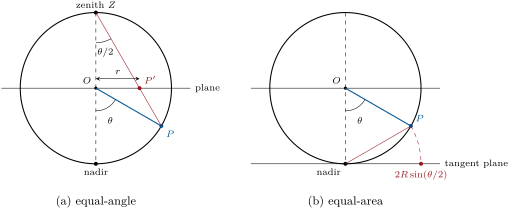
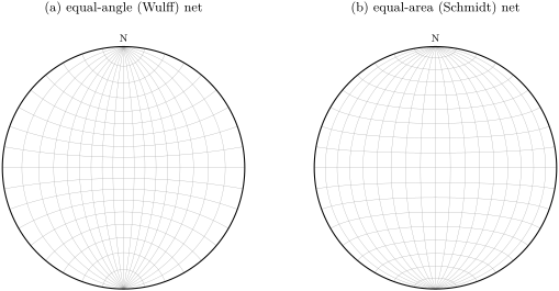
Planes, lines and angles. A plane of dip direction $\alpha$ and dip $\delta$ cuts the lower hemisphere along a half great circle. Its ends lie on the primitive at the two ends of the strike; its middle is the line of steepest dip, which plunges $\delta$ towards $\alpha$; and its pole lies $90{}^{\circ}$ from every point of it, in the azimuth $\alpha + 180{}^{\circ}$. A line in the plane is a point on the great circle. To plot data, a transparent overlay is laid on the net and turned about the centre until the data’s strike lies along the net’s north–south diameter; the great circle of the right dip is then traced, and the overlay is turned back. The angle between two lines is measured along the great circle through both points, counting the small-circle divisions it crosses, after turning the overlay until both points lie on one great circle of the net. The angle between two planes is the angle between their poles, or its supplement. A computer does the same with vectors: the angle between two lines of unit vectors $\vec u$ and $\vec v$ is $\arccos|\vec u\cdot\vec v|$.

Method 8.3 (Rotating data about an axis)

To undo a tilt, for instance to bring a bed back to the horizontal with the lineations that it carries, or to restore a palaeomagnetic direction measured in tilted strata (Chapter 4):

1. Choose the axis of rotation: for a tilted bed, its strike line, horizontal; the angle is the dip, in the sense that brings the bed up.
2. On the net, turn the overlay until the axis lies along the north–south diameter, where the small circles are the cones about it.
3. Move every point along its small circle by the angle of rotation, counted on the great circles. A point that would leave the lower hemisphere reappears at the opposite end of its small circle, in the opposite azimuth.
4. Turn the overlay back. With vectors, the rotation of $\vec v$ by the angle $\omega$ about the unit axis $\vec k$ is $\vec v' = \vec v \cos\omega + (\vec k\times\vec v)\sin\omega + \vec k(\vec k\cdot\vec v)(1 - \cos\omega)$.

8.2 Fold analysis

A cylindrical fold is generated by a straight line, the fold axis, moved parallel to itself. Every plane tangent to the folded surface contains the axis, so every normal to the surface is perpendicular to the axis: all the poles lie on the great circle of the plane perpendicular to the axis.

Definition 8.4 (Pi-diagram, beta-axis)

The pi-diagram of a fold is the plot of the poles of the planes measured on its folded surface. For a cylindrical fold they fall on a great circle, the $\pi$-girdle; the pole of the girdle is the beta-axis, the estimate of the fold axis given by the measurements.

With two limbs only, the beta-axis is the cross product of their normals, as the Year 1 volume showed for the hinge line. With two hundred scattered readings, a best fit is needed. The vector mean, which served for the readings of one plane, will not do: the poles of a girdle point every way along it, and their mean says little about the circle they lie on.

Definition 8.5 (Orientation tensor)

The orientation tensor of $N$ unit vectors $\vec p_1, \dots, \vec p_N$ is the symmetric matrix

$$T = \frac1N\sum_{i=1}^N \vec p_i\,\vec p_i^{\mathsf T}, \qquad T_{jk} = \frac1N\sum_i p_{ij}\,p_{ik} .$$

It does not change when a vector is replaced by its opposite, so it suits axes and poles, which have no sense. Its eigenvalues $\lambda_1 \ge \lambda_2 \ge \lambda_3 \ge 0$ add up to its trace, $1$.

Theorem 8.6 (Cluster and girdle from the orientation tensor)

For any unit vector $\vec u$,

$$\frac1N\sum_{i=1}^N (\vec p_i\cdot\vec u)^2 = \vec u^{\mathsf T}T\,\vec u ,$$

which takes its smallest value, $\lambda_3$, when $\vec u$ is the eigenvector $\vec e_3$ of the smallest eigenvalue, and its largest, $\lambda_1$, along the eigenvector $\vec e_1$. Since $\vec p_i\cdot\vec u$ is the sine of the angle between $\vec p_i$ and the plane perpendicular to $\vec u$, the great circle perpendicular to $\vec e_3$ is the girdle that minimises the sum of the squared sines of the distances of the poles to it, and $\sqrt{\lambda_3}$ is their root-mean-square sine. The axis $\vec e_1$ is the line closest to the vectors, the mean axis of a cluster.

The eigenvalues describe the shape of the data. A cluster has $\lambda_1$ near 1 and the other two small; a girdle has $\lambda_3$ near 0, the poles being spread along the circle so that $\lambda_1$ and $\lambda_2$ share the rest; uniformly scattered vectors give three eigenvalues near $1/3$. A fold is cylindrical, within the precision of the readings, when $\sqrt{\lambda_3}$ is no larger than the scatter of repeated readings of one plane. A conical fold, or two generations of folds, spread the poles away from any one great circle and raise $\lambda_3$.

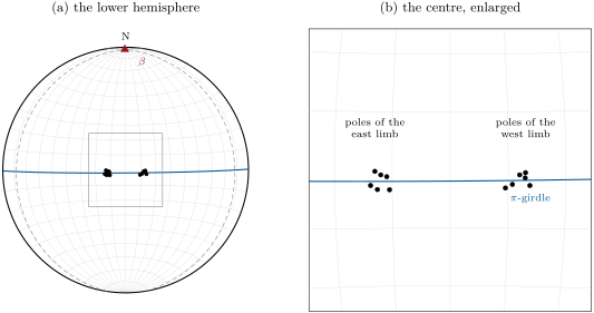
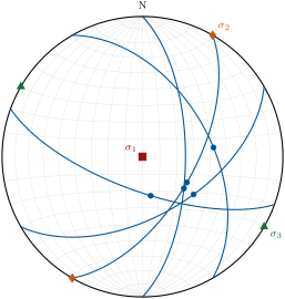
The figure below plots twelve readings from the two limbs of the Varden anticline, the series’ invented fold (Problem 8.1 computes its axis). The poles of the gentle limbs cluster near the centre of the net in two groups, which together define a girdle running almost east–west; the beta-axis lies on the primitive, almost due north. The mean planes of the two limbs, drawn as great circles, cross at the same point: the beta-axis is the line common to all the limbs.

8.3 Finite strain analysis

A deformed rock records its strain when it contains objects whose original shape, or whose original arrangement, is known: round ooids and reduction spots, fossils of known symmetry, pebbles, or simply the centres of grains that were once evenly spaced.

Definition 8.7 (Finite strain analysis, Fry method)

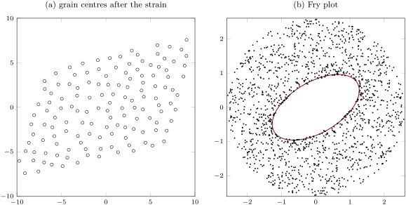
Finite strain analysis is the measurement of the strain ellipse, or ellipsoid, that a rock has undergone, from the shapes, orientations or spacings of objects whose state before the deformation is known. In the Fry method, the vector from the centre of every object to the centre of every other is plotted from one common origin; when the centres were spread with a minimum spacing and no preferred direction, the empty region around the origin is an ellipse of the shape and orientation of the strain ellipse.

Proposition 8.8 (The Fry void)

If a homogeneous strain maps every vector $\vec d$ to $F\vec d$, and no two centres were closer than $d_0$ before the strain, then after it the region around the origin of the Fry plot that is free of points contains the ellipse $\{F\vec d : |\vec d| < d_0\}$, of semi-axes $S_1d_0$ and $S_2d_0$ along the principal directions of the strain.

In practice the centres are not all at the minimum spacing, and the void is read as the inner edge of the densest ring of points; its ratio estimates the strain ratio $R_s = S_1/S_2$ slightly low. The figure below makes the test on an invented thin section, strained to $R_s = 2$ with the long axis at $30{}^{\circ}$ from the horizontal: the ellipse fitted to the edge of the void gives $R_s = 1.9$ and $30{}^{\circ}$. When the objects themselves are measured, initially round ones become ellipses of the axial ratio $R_s$ exactly; initially elliptical ones, with random orientations, end with ratios $R_f$ scattered about $R_s$, the largest when their long axes started parallel to the stretching direction, and their final orientations $\varphi$ gather around it. The plot of $R_f$ against $\varphi$, read with tables or a computer, separates the strain from the original shapes.

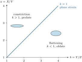
In three dimensions the strain ellipsoid has the principal stretches $X \ge Y \ge Z$. Its shape is plotted on the Flinn diagram, with $a = X/Y$ against $b = Y/Z$ and the parameter

On the line $k = 1$, which holds plane strain at constant volume ($Y = 1$, $X = 1/Z$, so $a = b$), the ellipsoid is neither cigar nor pancake. Above it, $k > 1$, the ellipsoid is prolate, stretched in one direction by a constriction: rocks deformed this way grow a strong lineation. Below, $k < 1$, it is oblate, flattened, and the rock grows a strong foliation.

8.4 Palaeostress

Anderson’s theory says on which planes new faults form, and that they slip perpendicular to $\sigma_2$. Most faults, though, are older weaknesses reactivated in a stress field that they did not choose, and they slip obliquely. Their slip directions, read on the striations of the fault surfaces, still record the stress, if each fault slips the way the stress pushes it.

Definition 8.9 (Palaeostress, Wallace–Bott hypothesis, stress ratio, fault-slip inversion)

Palaeostress is the state of stress that acted in a rock in the past, as far as it can be deduced from the structures it left: in practice, the directions of the principal stresses and the stress ratio

$$\Phi = \frac{\sigma_2 - \sigma_3}{\sigma_1 - \sigma_3}, \qquad 0 \le \Phi \le 1 .$$

The Wallace–Bott hypothesis states that a fault slips parallel to the shear stress resolved on its plane by a uniform stress, each fault independently. A fault-slip inversion is the search for the principal directions and the stress ratio whose predicted slip directions best fit a set of measured faults and striations.

Theorem 8.10 (Slip direction on a plane)

Let $S$ be the stress tensor, compressions counted positive, and $\vec n$ the upward unit normal of a fault. Write

$$\vec\tau = S\vec n - (\vec n\cdot S\vec n)\,\vec n .$$

Under the Wallace–Bott hypothesis the hanging wall slips relative to the footwall along $-\vec\tau$, the shear traction that it exerts on the footwall. Moreover:

1. the direction of $\vec\tau$ is unchanged when $S$ is replaced by $aS + bI$ with $a > 0$; it therefore depends only on the principal directions and on $\Phi$, and the reduced tensor $S' = \mathrm{diag}(1, \Phi, 0)$ in the principal frame $(\vec e_1, \vec e_2, \vec e_3)$ predicts the same slip as $S$;
2. if $\vec n$ is perpendicular to one principal direction, the slip is perpendicular to it too;
3. with $n_k = \vec n\cdot\vec e_k$, the direction is that of $\vec\tau' = \vec\tau_0 + \Phi\,\vec\tau_1$, linear in $\Phi$, where $\vec\tau_0 = n_1(\vec e_1 - n_1\vec n)$ and $\vec\tau_1 = n_2(\vec e_2 - n_2\vec n)$.

Part (b) is Anderson’s case: a fault that contains $\sigma_2$ slips perpendicular to it, whatever $\Phi$, so that it says nothing of the stress ratio. Part (c) turns a measured slip into $\Phi$. Let $\vec u$ be the unit slip vector of the hanging wall, from the rake, and $\vec w = \vec n\times\vec u$ the direction in the plane perpendicular to it. The predicted slip is parallel to $\vec u$ when $(\vec\tau_0 + \Phi\vec\tau_1)\cdot\vec w = 0$, and since $\vec n\cdot\vec w = 0$,

provided the predicted slip then points along $+\vec u$ and not $-\vec u$.

When the principal directions are not known, each fault gives one equation, the angle of its slip within its plane, for four unknowns: three angles that orient the principal axes, and $\Phi$. Four faults of different attitudes are the minimum, and a few tens are usual. The inversion minimises the sum of the squared angles between the measured and the predicted slips, by least squares on a grid or by iteration as in Section 1.4. Faults that do not fit form a second population, perhaps of another age.

The figure below shows five faults of the Varden Hills: the main normal fault and four smaller ones, all with normal slip. A grid search over $\Phi$ and the trend of $\sigma_3$, with $\sigma_1$ vertical, fits all five within a quarter of a degree, with $\sigma_3$ horizontal towards $120{}^{\circ}$.

The P and T axes of the Year 1 volume are not the principal stresses. They are built from the fault plane and the slip alone, at $45{}^{\circ}$ from the plane in the plane that contains the slip and the normal; a new fault, in rock with an angle of friction near $30{}^{\circ}$, makes about $30{}^{\circ}$ with $\sigma_1$, and a reactivated one any angle. One mechanism gives the P and T axes; only many faults of different attitudes, inverted together, give the stress. The hypothesis itself has limits: the stress may vary from fault to fault, blocks may rotate, and faults that meet hinder each other’s slip.

8.5 Restoring a cross-section

A cross-section is an interpretation: between the surface and the boreholes, the geologist draws what is likely. The Year 2 volume, in its chapter on the Alps, called a section balanced when it can be returned to an undeformed state with the lengths of the beds and the areas of the units conserved, folds and thrusts rooting on a décollement. Restoring is the test.

Definition 8.11 (Section restoration, pin line, kink-band method)

Section restoration undoes, on a cross-section drawn parallel to the direction of tectonic transport, the deformation it shows, event by event in the reverse order, keeping the lengths of the beds and the areas of the units in the plane of the section. A pin line is a line across the beds, placed where they did not slip along each other (in the undeformed foreland, or on the axial surface of a symmetric fold), which is taken to be perpendicular to the beds in the restored section; lengths are measured from it. In the kink-band method the folds are drawn as straight limbs of constant bed thickness joined at sharp hinges, whose axial surfaces bisect the angle between the limbs; each bed is then a broken line, whose length is the sum of its straight segments.

A bed folded into straight limbs dipping $\delta$ either way, over the horizontal distance $L$, has the length $L/\cos\delta$: its shortening is $S = L(1/\cos\delta - 1)$, the relative change of length $\cos\delta - 1$. Areas give the other half of the balance.

Proposition 8.12 (Depth to detachment)

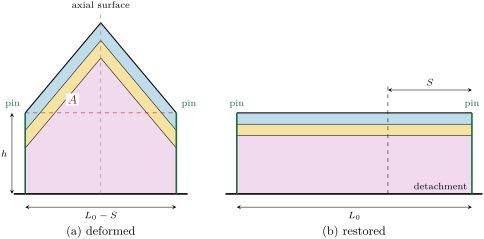
Let a layer at the height $h$ above a horizontal detachment be shortened by $S$ in the plane of a section, and let the rock between it and the detachment keep its area, with no material crossing the ends of the section. Then the area $A$ by which the folded layer stands above its original level satisfies

$$A = S\,h , \qquad\text{so that}\qquad h = \frac AS .$$

Two layers give both unknowns: their excess areas differ by $S$ times their vertical separation. The figure below sets out the construction.

A section crossed by a fault is restored in the reverse order of the events: the youngest structure first. A normal fault of throw $t_h$ and dip $\delta$ has the heave $t_h/\tan\delta$ and the slip $t_h/\sin\delta$ on a section parallel to its dip; the hanging wall is moved back up the fault by the slip. On a section oblique to the slip, both the dip of the fault and its displacement are apparent, and a section that seems to balance may not: this is why sections are drawn parallel to the transport direction.

In the field — Measuring an attitude

To measure a bedding plane, the geologist lays the open lid of a compass-clinometer flat against the surface, chosen smooth and representative, and turns the body until its bubble shows it level: the needle then gives the dip direction, and the clinometer, with the instrument turned on its edge along the steepest line, the dip. The reading is noted as dip direction and dip, for instance $075/13$, with the place and the kind of surface. Azimuths read with a magnetic needle are corrected for the local declination. A smartphone with a geology application measures the same thing in one step: held flat against the plane, its accelerometers give the direction of gravity and hence the dip, and its magnetometer the azimuth. Field geologists compare it regularly with a compass, since nearby iron and the phone’s own circuits can disturb the magnetometer; they repeat each reading and average the normals with the vector mean.

8.6 Exercises

Exercise 8.1 ★

Give the trend and plunge of the pole of the plane $040/30$ (dip direction, dip). Give the attitude of the plane whose pole trends $315{}^{\circ}$ and plunges $20{}^{\circ}$.

Solution

Solution of Exercise 8.1.

The pole trends $40 + 180 = 220{}^{\circ}$ and plunges $90 - 30 = 60{}^{\circ}$. The plane dips $90 - 20 = 70{}^{\circ}$ towards $315 - 180 = 135{}^{\circ}$: $135/70$.

Exercise 8.2 ★

A line plunges $30{}^{\circ}$. At what distance from the centre does it plot on an equal-angle net and on an equal-area net, both of radius $10\,\mathrm{cm}$?

Solution

Solution of Exercise 8.2.

$\theta = 60{}^{\circ}$. Equal-angle: $10\tan30{}^{\circ} = 5.77\,\mathrm{cm}$; equal-area: $10\sqrt2\sin30{}^{\circ} = 7.07\,\mathrm{cm}$.

Exercise 8.3 ★

The limbs of a fold have the attitudes $090/30$ and $270/30$. Compute the angle between their poles with the dot product of the normals, the interlimb angle, and the class of the fold.

Solution

Solution of Exercise 8.3.

$\vec n_1 = (\sin30{}^{\circ}, 0, \cos30{}^{\circ})$, $\vec n_2 = (-\sin30{}^{\circ}, 0, \cos30{}^{\circ})$, $\vec n_1\cdot\vec n_2 = -0.25 + 0.75 = 0.5$: the poles are $60{}^{\circ}$ apart, the interlimb angle is $120{}^{\circ}$, an open fold.

Exercise 8.4 ★

A fault $090/60$ carries striations of rake $-45{}^{\circ}$. With the strike vector $\vec s = (0, 1, 0)$ and the down-dip vector $\vec d$ of the plane, the slip of the hanging wall is $\vec u = \cos r\,\vec s - \sin r\,\vec d$. Compute $\vec d$, $\vec u$, and the trend and plunge of the slip. Name the fault.

Solution

Solution of Exercise 8.4.

$\vec d = (\cos60{}^{\circ}, 0, -\sin60{}^{\circ}) = (0.5, 0, -0.866)$ and $\vec u = 0.707\,\vec s + 0.707\,\vec d = (0.354, 0.707, -0.612)$: trend $\operatorname{atan2}(0.354, 0.707) = 26.6{}^{\circ}$, plunge $\arcsin0.612 = 37.8{}^{\circ}$. The rake lies between $-90{}^{\circ}$ (normal) and 0 (sinistral): an oblique normal fault with a sinistral component.

Exercise 8.5 ★★

The limbs of a fold have the attitudes $060/40$ and $250/30$. Compute the trend and plunge of its axis, and its interlimb angle.

Solution

Solution of Exercise 8.5.

$$\begin{gather*} \vec n_1 = (0.5567, 0.3214, 0.7660),\qquad \vec n_2 = (-0.4698, -0.1710, 0.8660),\\ \vec n_1\times\vec n_2 = (0.4093, -0.8420, 0.0558), \end{gather*}$$

of length $0.9379$. Its opposite, $-\vec n_1\times\vec n_2$, points down: trend $334.1{}^{\circ}$, plunge $\arcsin(0.0558/0.9379) = 3.4{}^{\circ}$. $\vec n_1\cdot\vec n_2 = 0.3469$, $69.7{}^{\circ}$ between the normals, interlimb angle $110.3{}^{\circ}$: an open fold.

Exercise 8.6 ★★

Compute the fraction of the area of the net that lies inside the circle of lines plunging more than $60{}^{\circ}$, on the equal-area and on the equal-angle net, and the fraction of the directions of the lower hemisphere that plunge more than $60{}^{\circ}$. Which net should be used to count poles?

Solution

Solution of Exercise 8.6.

Plunge above $60{}^{\circ}$ means $\theta < 30{}^{\circ}$. Equal-area: $r^2 = 2\sin^215{}^{\circ} = 0.134$, $13.4\,\%$ of the net; equal-angle: $\tan^215{}^{\circ} = 0.072$, $7.2\,\%$. On the sphere the cap holds $1 - \cos30{}^{\circ} = 0.134$ of the hemisphere: only the equal-area net shows it with its true share, so poles are counted on it.

Exercise 8.7 ★★

Three poles lie in the vertical east–west plane, at $-20{}^{\circ}$, $0$ and $20{}^{\circ}$ from the vertical: $\vec p = (\sin a, 0, -\cos a)$. Compute their orientation tensor, its eigenvalues and eigenvectors, and the beta-axis. Why is the smallest eigenvalue exactly zero?

Solution

Solution of Exercise 8.7.

$$\begin{gather*} T_{xx} = \frac{2\sin^220{}^{\circ}}3 = 0.078,\qquad T_{zz} = \frac{2\cos^220{}^{\circ} + 1}3 = 0.922,\\ T_{xz} = -\frac{\sin20{}^{\circ}\cos20{}^{\circ} - \sin20{}^{\circ}\cos20{}^{\circ}}3 = 0, \end{gather*}$$

and every term with $y$ is 0. The eigenvalues are $0.922$ (vertical), $0.078$ (east) and $0$ (north): the beta-axis is horizontal, north–south. The three poles lie in one plane, so none has a component along its normal, and $\vec u^{\mathsf T}T\vec u = 0$ for $\vec u$ along it.

Exercise 8.8 ★★

Place on the Flinn diagram the ellipsoid $X : Y : Z = 3 : 1.5 : 1$, then the ellipsoid of constant volume with $X = 1.8$ and $Y = 1.1$. Compute $k$ for each and name the strain.

Solution

Solution of Exercise 8.8.

$a = 2$, $b = 1.5$, $k = 1/0.5 = 2$: constriction. $Z = 1/(1.8\times1.1) = 0.505$, $a = 1.636$, $b = 2.178$, $k = 0.636/1.178 = 0.54$: flattening.

Exercise 8.9 ★★

In a section cut parallel to the stretching, initially round ooids are ellipses of axial ratio $2.25$, all parallel, and the area of each is unchanged. Compute the principal stretches and the extension along the long axis. Before the strain, the ooid centres were never closer than $0.4\,\mathrm{mm}$: give the semi-axes of the void of the Fry plot.

Solution

Solution of Exercise 8.9.

$S_1/S_2 = 2.25$ and $S_1S_2 = 1$: $S_1 = 1.5$, $S_2 = 0.667$; the long axis was extended by $50\,\%$. The void has the semi-axes $1.5\times0.4 = 0.60\,\mathrm{mm}$ and $0.667\times0.4 = 0.27\,\mathrm{mm}$.

Exercise 8.10 ★★★

At $\theta = 60{}^{\circ}$ from the nadir, compute the stretch along the radius, $\mathrm dr/(R\,\mathrm d\theta)$, and around the circle, $r/(R\sin\theta)$, for both projections. Check the theorem on the projections, and give the ratio of the axes of the oval into which the equal-area net turns a very small circle there.

Solution

Solution of Exercise 8.10.

Equal-angle: $1/(2\cos^230{}^{\circ}) = 0.667$ along the radius and $\tan30{}^{\circ}/\sin60{}^{\circ} = 0.577/0.866 = 0.667$ around: equal, conformal. Equal-area: $\mathrm dr/(R\,\mathrm d\theta) = (\sqrt2/2)\cos30{}^{\circ} = 0.612$ and $\sqrt2\sin30{}^{\circ}/\sin60{}^{\circ} = 0.707/0.866 = 0.816$; the product is $0.500$, the area factor of the theorem. A small circle becomes an oval of axes in the ratio $0.816/0.612 = 1.33$, long around the centre.

Exercise 8.11 ★★★

In a strike-slip regime, $\sigma_1$ is horizontal towards $000{}^{\circ}$, $\sigma_3$ horizontal towards $090{}^{\circ}$ and $\sigma_2$ vertical. A vertical fault strikes $020{}^{\circ}$. Without computing $\vec\tau$, show that its slip is horizontal for every $\Phi$. Then compute $-\vec\tau$ for $\Phi = 0.4$ with the plane’s normal $\vec n = (\cos20{}^{\circ}, -\sin20{}^{\circ}, 0)$ and give the sense of slip.

Solution

Solution of Exercise 8.11.

The fault is vertical, so its normal is horizontal and perpendicular to the vertical $\sigma_2$; by part (b) of the theorem the slip is perpendicular to $\sigma_2$, horizontal, for every $\Phi$. With $\sigma_1 = 1$ along north, $\sigma_3 = 0$ along east: $S\vec n = (0, -0.342, 0)$, $\vec n\cdot S\vec n = 0.117$, $\vec\tau = (0, -0.342, 0) - 0.117\,(0.940, -0.342, 0) = (-0.110, -0.302, 0)$ and $-\vec\tau = (0.110, 0.302, 0)$, towards $020{}^{\circ}$. The block on the side of $\vec n$, the east side, moves north-north-east along the strike: seen from the west side, it moves to the left, a sinistral fault (rake 0). $\sigma_2$ did not enter the computation.

Exercise 8.12 ★★★

A section $20\,\mathrm{km}$ long crosses a train of detachment folds. Two horizons $1.0\,\mathrm{km}$ apart stand above their original levels by the areas $6.0\,\mathrm{km}^{2}$ (lower) and $7.5\,\mathrm{km}^{2}$ (upper). Compute the shortening, the depth of the detachment below the lower horizon, the original length of the section and its relative change of length.

Solution

Solution of Exercise 8.12.

$S = (7.5 - 6.0)/1.0 = 1.5\,\mathrm{km}$; $h = 6.0/1.5 = 4.0\,\mathrm{km}$ below the lower horizon. The section was $20 + 1.5 = 21.5\,\mathrm{km}$ long, and changed by $-1.5/21.5 = -7.0\,\%$.

8.7 Problem: Folds and Faults of the Varden Hills

Problem 8.1

Weekend problem — the axis of a fold, the stress of a fault set and the restoration of a section, in an invented region

In the Varden Hills, the series’ invented region, a Mesozoic cover rests on a basement of schist and granite. The cover is folded into an upright anticline and syncline with straight limbs, then cut by a normal fault. A geologist measured twelve bedding planes on the two limbs of the anticline (dip direction/dip, in degrees):

east limb	075/13	084/11	089/13	079/14	086/12	072/11
west limb	283/11	272/13	281/14	288/10	276/13	274/12

The sums of the upward unit normals of the six readings of each limb are $\vec S_E = (1.2583, 0.2017, 5.8604)$ and $\vec S_W = (-1.2445, 0.1886, 5.8636)$ (east, north, up). Five faults carry striations (dip direction/dip, rake of the hanging wall’s slip): $120/60/{-90}$ (the main fault), $150/55/{-76}$, $090/65/{-108}$, $200/70/{-78}$ and $060/50/{-105}$. The main fault has a throw of $200\,\mathrm{m}$. The anticline and syncline axes are $4\,\mathrm{km}$ apart, so that the folds repeat every $8\,\mathrm{km}$ from east to west.

Part I — Poles and the beta-axis.

1. Give the trend and plunge of the pole of the reading $075/13$, and its distance from the centre of an equal-area net of radius $10\,\mathrm{cm}$.
2. Compute the upward unit normal of the reading $075/13$; check it against $\vec S_E$ in size.
3. Compute the mean attitude of each limb from $\vec S_E$ and $\vec S_W$, the mean resultant lengths, and the root-mean-square scatter of the readings about their means.
4. Compute $\vec S_E\times\vec S_W$, and the trend and plunge of the beta-axis.
5. Compute the angle between the two mean normals, the interlimb angle, and the class of the fold.
6. The axial plane of this symmetric fold contains the beta-axis and is perpendicular to $\vec m_E - \vec m_W$, the difference of the mean unit normals. Give its attitude; is the fold upright?
7. Give the attitude of the $\pi$-girdle, and say why the poles lie on it.

Part II — The orientation tensor. The orientation tensor of the twelve poles is

$$T = \begin{pmatrix} 0.04400 & 0.00035 & 0.00109\\ 0.00035 & 0.00144 & 0.03179\\ 0.00109 & 0.03179 & 0.95456 \end{pmatrix},$$

with the eigenvalues $0.95562$, $0.04400$ and $0.00038$.

8. Check that the trace of $T$ is 1. With $\vec b = (0.0053, -0.9994, 0.0333)$, the unit vector along $\vec S_E\times\vec S_W$, compute $\vec b^{\mathsf T}T\vec b$. What does the result say about $\vec b$?
9. Compute the root-mean-square angle between the poles and the girdle.
10. Explain the value of $\lambda_2$ from the dips of the limbs.
11. Is the fold cylindrical within the precision of the readings?
12. The plunge of the beta-axis is set by the north–south tilt of the girdle, to which each pole contributes with the scatter found in question 9. Estimate the standard error of the plunge.

Part III — The palaeostress.

13. What kind of fault is the main fault? Following Anderson, give the directions of $\sigma_1$, $\sigma_2$ and $\sigma_3$.
14. Show, with the theorem on the slip direction, that the main fault slips straight down its dip for every value of $\Phi$. What does it tell of $\Phi$?
15. For the fault $150/55$, compute $\vec n$ and its components $n_1 = \vec n\cdot\vec e_1$ and $n_2 = \vec n\cdot\vec e_2$, with $\vec e_1$ vertical and $\vec e_2$ horizontal towards $030{}^{\circ}$.
16. Its slip gives $\vec w = \vec n\times\vec u = (0.771, 0.605, 0.198)$. Compute $\Phi$.
17. The other three small faults give $\Phi = 0.294$, $0.301$ and $0.306$. Give the mean, and say where the spread comes from.
18. What does $\Phi = 0.3$ say of $\sigma_2$?
19. Compute the P and T axes of the main fault (at $45{}^{\circ}$ from the plane, in its dip plane), and compare them with $\sigma_1$ and $\sigma_3$.

Part IV — Restoring an east–west section.

20. Compute the apparent dip of the east limb, $080.9/12.3$, on an east–west section.
21. Taking the limbs at $12{}^{\circ}$ on the section, compute the restored length of one fold wavelength, the shortening and the relative change of length.
22. Compute the height of the anticline crest above the synclines and the excess area of one wavelength, assuming that the synclines stayed at the original level.
23. Compute the depth of the detachment beneath the folded bed. Can the folds be detached at the base of the cover, a few hundred metres down?
24. Compute the heave and the slip of the main fault on a section along $120{}^{\circ}$.
25. On the east–west section, compute the apparent dip of the fault and its apparent heave. Which section should be restored?
26. In what order are the fault and the folds restored, and where are the pin lines placed?
27. What is the plunge of the Varden fold axis, recovered from the twelve readings?

Solution

Solution of Problem 8.1.

1. The pole trends $255{}^{\circ}$ and plunges $77{}^{\circ}$; $\theta = 13{}^{\circ}$ and $r = 10\sqrt2\sin6.5{}^{\circ} = 1.60\,\mathrm{cm}$ from the centre, towards $255{}^{\circ}$.

2. $\vec n = (\sin13{}^{\circ}\sin75{}^{\circ}, \sin13{}^{\circ}\cos75{}^{\circ}, \cos13{}^{\circ}) = (0.2173, 0.0582, 0.9744)$. Six nearly parallel unit vectors add up to nearly 6: $|\vec S_E| = 5.9974$.

3. East limb: $\bar\alpha = \operatorname{atan2}(1.2583, 0.2017) = 80.9{}^{\circ}$ and $\bar\delta = \arccos(5.8604/5.9974) = 12.3{}^{\circ}$; $\bar R = 5.9974/6 = 0.99956$ and the scatter is $\sqrt{2\times0.00044} = 0.0297\,\mathrm{rad}$, or $1.7{}^{\circ}$. West limb: $\bar\alpha = \operatorname{atan2}(-1.2445, 0.1886) = 278.6{}^{\circ}$ and $\bar\delta = \arccos(5.8636/5.9972) = 12.1{}^{\circ}$; $\bar R = 0.99953$, scatter $1.8{}^{\circ}$.

4.

$$\vec S_E\times\vec S_W = (0.0774, -14.6714, 0.4883),$$

of length $14.680$. Its opposite points down: the trend is $\operatorname{atan2}(-0.0774, 14.6714) = 359.7{}^{\circ}$ and the plunge $\arcsin(0.4883/14.680) = 1.9{}^{\circ}$.

5. The cosine of the angle between the mean normals is $32.835/35.968 = 0.9129$, the dot product of the sums divided by their lengths: $24.1{}^{\circ}$ between the normals, an interlimb angle of $155.9{}^{\circ}$: an open fold, close to gentle.

6.

$$\begin{gather*} \vec m_E = (0.2098, 0.0336, 0.9772),\qquad \vec m_W = (-0.2075, 0.0314, 0.9777),\\ \vec m_E - \vec m_W = (0.4173, 0.0022, -0.0005): \end{gather*}$$

a horizontal normal towards $089.7{}^{\circ}$. The axial plane is vertical, striking $359.7{}^{\circ}$, practically north–south: the fold is upright.

7. The girdle is the plane whose pole is the beta-axis: dip direction $179.7{}^{\circ}$, dip $90 - 1.9 = 88.1{}^{\circ}$, almost the east–west vertical plane. Every limb contains the fold axis, so every normal is perpendicular to it and lies in the plane perpendicular to it.

8. $0.04400 + 0.00144 + 0.95456 = 1.00000$. $\vec b^{\mathsf T}T\vec b = 0.00038$, the smallest eigenvalue: $\vec b$ is, to the rounding, the eigenvector $\vec e_3$, and the girdle through the two mean poles is the best-fit girdle of all twelve.

9. $\arcsin\sqrt{0.00038} = \arcsin0.0195 = 1.1{}^{\circ}$.

10. Along the girdle the poles sit about $12.2{}^{\circ}$ from the vertical, on either side; $\sin^212.2{}^{\circ} = 0.045$, the mean square of their east–west components, which is $\lambda_2$.

11. Yes: the poles stray from the girdle by $1.1{}^{\circ}$ on average, no more than the $1.7{}^{\circ}$ scatter of the readings of one limb about their mean.

12. $1.1{}^{\circ}/\sqrt{12} = 0.3{}^{\circ}$: the plunge is $1.9{}^{\circ}$ $\pm$ $0.3{}^{\circ}$.

13. A rake of $-90{}^{\circ}$: a pure normal fault, dip-slip. Anderson: $\sigma_1$ vertical, $\sigma_3$ horizontal along the dip direction, $120{}^{\circ}$–$300{}^{\circ}$, $\sigma_2$ horizontal along the strike, $030{}^{\circ}$–$210{}^{\circ}$.

14. The normal of $120/60$ lies in the vertical plane trending $120{}^{\circ}$, which holds $\vec e_1$ and $\vec e_3$: $n_2 = 0$. By part (b) the slip is perpendicular to $\sigma_2$, the strike, for every $\Phi$: it is dip-slip. The fault tells nothing of $\Phi$; in the formula both $n_2$ and $\vec e_2\cdot\vec w$, hence numerator and denominator, vanish.

15. $\vec n = (\sin55{}^{\circ}\sin150{}^{\circ}, \sin55{}^{\circ}\cos150{}^{\circ}, \cos55{}^{\circ}) = (0.4096, -0.7094, 0.5736)$; $n_1 = 0.574$; $n_2 = 0.5\times 0.4096 + 0.866\times(-0.7094) = -0.410$.

16. $\vec e_1\cdot\vec w = 0.198$ and $\vec e_2\cdot\vec w = 0.5\times 0.771 + 0.866\times0.605 = 0.909$, so $\Phi = -(0.574\times0.198)/(-0.410\times 0.909) = 0.1137/0.3727 = 0.305$.

17. $(0.305 + 0.294 + 0.301 + 0.306)/4 = 0.30$. The rakes were rounded to the degree; one degree of rake moves $\Phi$ by about 0.02 on these faults, so the half-degree of rounding explains the spread.

18. $\sigma_2 - \sigma_3 = 0.3(\sigma_1 - \sigma_3)$: $\sigma_2$ is closer to $\sigma_3$ than to $\sigma_1$. Both horizontal stresses are well below the vertical one; the region was extended mostly towards $120{}^{\circ}$, a little along $030{}^{\circ}$.

19. With $\vec n = (0.750, -0.433, 0.500)$ and the slip $\vec u = (0.433, -0.250, -0.866)$, $(\vec n - \vec u)/\sqrt2$ plunges $75{}^{\circ}$ towards $300{}^{\circ}$: P; $(\vec n + \vec u)/\sqrt2$ plunges $15{}^{\circ}$ towards $120{}^{\circ}$: T. They lie in the same vertical plane as $\sigma_1$ and $\sigma_3$ but $15{}^{\circ}$ away from them, because the fault makes $30{}^{\circ}$, not $45{}^{\circ}$, with $\sigma_1$.

20. $\tan a = \tan12.3{}^{\circ}\times\cos(90{}^{\circ} - 80.9{}^{\circ}) = 0.2180\times0.9874 = 0.2153$: $a = 12.1{}^{\circ}$.

21. $L_0 = 8000/\cos12{}^{\circ} = 8178.7\,\mathrm{m}$, $S = 178.7\,\mathrm{m}$, a relative change of $\cos12{}^{\circ} - 1 = -2.2\,\%$.

22. $4000\tan12{}^{\circ} = 850.2\,\mathrm{m}$; $A = \tfrac12\times8000\times 850.2 = 3.40 \times 10^{6}\,\mathrm{m}^{2}$.

23. $h = 3.40 \times 10^{6}/178.7 = 19.0\,\mathrm{km}$. A detachment at the base of the cover would give $h$ of a few hundred metres and an excess area some fifty times smaller: the folds are not detached there. Either the basement folded with the cover, or the synclines sank below the original level, which makes $A$ smaller; the section alone cannot tell.

24. Heave $200/\tan60{}^{\circ} = 115.5\,\mathrm{m}$, slip $200/\sin60{}^{\circ} = 230.9\,\mathrm{m}$.

25. $\tan a = \tan60{}^{\circ}\cos30{}^{\circ} = 1.500$: $a = 56.3{}^{\circ}$, and the apparent heave is $200/1.5 = 133.3\,\mathrm{m}$. The slip of the fault is down the dip, towards $120{}^{\circ}$: the section along $120{}^{\circ}$ shows true lengths and should be the one restored.

26. The fault cuts the folds, so it is younger and is restored first, moving the hanging wall back up the fault by $230.9\,\mathrm{m}$; the folds are then unfolded. The pin lines go on the axial surfaces of the synclines, in the footwall, where the symmetric folds had no slip between the beds.

27. The Varden fold axis plunges $1.9{}^{\circ}$ towards the north (trend $359.7{}^{\circ}$): the $2{}^{\circ}$ built into the region, recovered to the $0.3{}^{\circ}$ that twelve readings allow.