20Atmospheric Dynamics

On a winter map of the upper troposphere the jet stream does not circle the pole as a smooth ring. It meanders, in a few great waves round the hemisphere, troughs reaching towards the subtropics and ridges towards the pole, and at the surface depressions are born, grow for a few days and die under them. The waves drift slowly, sometimes against the wind that carries them. Their number, their speed and the growth of the storms beneath them follow from one conserved quantity, the vorticity of the air seen from space, and from the energy stored in the temperature contrast between the tropics and the poles.

You already know

Vorticity and circulation are in the physics books. The Rossby waves of the upper troposphere, troughs and ridges, the extratropical cyclone and the principle of numerical weather prediction are described in the Year 2 volume, in its chapter on weather systems. The Hadley, Ferrel and polar cells, the jets, the westerlies and the angular-momentum wind of a ring of air are in the Year 1 volume, in its chapter on the general circulation of the atmosphere, and the poleward transport of heat in its chapter on radiation and heat transport. The Coriolis parameter $f$, the $\beta$-plane, the Rossby radius and the thermal wind are in Chapter 19.

20.1 Vorticity

The vorticity of a fluid, the curl of its velocity, is twice its local angular velocity. For the large-scale atmosphere only its vertical component matters, and the rotation of the Earth contributes to it.

Definition 20.1 (Relative, planetary and absolute vorticity)

For a horizontal velocity $(u, v)$, the relative vorticity is the vertical component of the curl of the velocity relative to the ground, $\zeta = \partial v/\partial x - \partial u/\partial y$, positive for anticlockwise rotation seen from above. The planetary vorticity is the vertical component of the vorticity of the Earth’s rotation, $2\Omega\sin\varphi = f$. The absolute vorticity is their sum, $\zeta + f$.

In the Northern Hemisphere a depression, where the air turns anticlockwise, has $\zeta > 0$ and is called cyclonic; an anticyclone has $\zeta < 0$. A wind of $15\,\mathrm{m}/\mathrm{s}$ turning on a circle of $1000\,\mathrm{km}$ has $\zeta = 2V/R = 3 \times 10^{-5}\,\mathrm{s}^{-1}$ in solid rotation, a third of $f$ at $45{}^{\circ}$: the planetary part is usually the larger.

Theorem 20.2 (Barotropic vorticity equation)

In an inviscid, two-dimensional flow without horizontal divergence on a $\beta$-plane, the absolute vorticity of each parcel is conserved:

$$\frac{\mathrm D(\zeta + f)}{\mathrm Dt} = 0 , \qquad\text{that is}\qquad \frac{\partial\zeta}{\partial t} + u\frac{\partial\zeta}{\partial x} + v\frac{\partial\zeta}{\partial y} + \beta v = 0 .$$

This is the barotropic vorticity equation.

The proof also gave the general law, $\mathrm D(\zeta + f)/\mathrm Dt = -(\zeta + f)\delta$: convergence spins a column up, divergence spins it down, like a skater pulling in or spreading her arms. In a layer whose depth changes, convergence is tied to the stretching of the column, and the conserved quantity becomes a ratio.

Definition 20.3 (Potential vorticity)

The potential vorticity of a column of a homogeneous layer of depth $h$ is $q = (\zeta + f)/h$. In a continuously stratified fluid, Ertel’s potential vorticity is $q = (\vec\omega_a\cdot \nabla\theta)/\rho$, with $\vec\omega_a$ the absolute vorticity vector and $\theta$ the potential temperature.

Theorem 20.4 (Conservation of potential vorticity)

In a homogeneous, hydrostatic, inviscid layer of variable depth $h$ whose horizontal velocity does not vary with height, $\mathrm Dq/\mathrm Dt = 0$ for $q = (\zeta + f)/h$.

Ertel’s form is conserved in the same way by an adiabatic, frictionless flow of a stratified fluid, with the distance between two surfaces of constant $\theta$ playing the part of $h$. A column of air crossing a mountain range is squeezed on the way up: its absolute vorticity falls, it turns anticyclonically over the crest, and it stretches and turns cyclonically in the lee. Conservation of absolute or potential vorticity is the restoring mechanism of the waves of the next section, as the figure below shows.

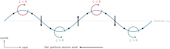
20.2 Rossby waves

The Year 2 volume described the Rossby waves of the upper troposphere. The barotropic vorticity equation explains them. Write the flow as a uniform westerly $U$ plus a small disturbance with streamfunction $\psi'$, so that $u' = -\partial\psi'/\partial y$, $v' = \partial\psi'/\partial x$ and $\zeta' = \nabla^2\psi'$.

Theorem 20.5 (Dispersion of Rossby waves)

Small disturbances $\psi' \propto \mathrm e^{\mathrm i(kx + ly - \omega t)}$ of a uniform westerly $U$ on a $\beta$-plane obey the Rossby-wave dispersion relation

$$\omega = Uk - \frac{\beta k}{k^2 + l^2} .$$

Their eastward phase speed is $c = \omega/k = U - \beta/K^2$, with $K^2 = k^2 + l^2$, and their eastward group velocity $c_g = \partial\omega/\partial k = U + \beta(k^2 - l^2)/K^4$.

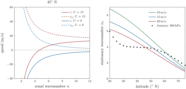
Relative to the air, the waves always move west, the faster the longer they are. A westerly wind carries the short waves east; the long ones it cannot carry, and they drift west against it. In between, one length stands still.

Proposition 20.6 (Stationary Rossby waves)

In a westerly $U > 0$, a wave with no meridional structure ($l = 0$) is stationary when its wavelength is the stationary Rossby wavelength $\lambda_s = 2\pi\sqrt{U/\beta}$. Round the latitude circle $\varphi$ this is a whole number of waves close to $n_s = \sqrt{2\Omega a\cos^3\varphi/U}$.

At $45{}^{\circ}$ N in a westerly of $15\,\mathrm{m}/\mathrm{s}$, with $\beta = 1.62 \times 10^{-11}\,\mathrm{m}^{-1}\,\mathrm{s}^{-1}$, $\lambda_s = 6050\,\mathrm{km}$ and $n_s = 4.7$: four or five waves round the hemisphere. With the zonal-mean January wind at $300\,\mathrm{hPa}$, about $21\,\mathrm{m}/\mathrm{s}$ at $45{}^{\circ}$ N, $n_s$ is about four from $35{}^{\circ}$ to $55{}^{\circ}$ N, falling poleward. The group velocity of a wave with $l = 0$ exceeds its phase speed by $2\beta/k^2$: energy runs ahead of the wave, so a disturbance set off at one place builds new troughs and ridges downstream of it, a few days later and thousands of kilometres east, while the pattern itself barely moves. Mountain ranges and the contrasts of temperature between continents and oceans force stationary waves of exactly this kind, through the stretching and squeezing of potential vorticity.

20.3 Baroclinic instability

The waves of the last section are neutral: they neither grow nor decay. The storms of the middle latitudes grow, and draw their energy from the temperature contrast that the thermal wind expresses.

Definition 20.7 (Available potential energy)

The available potential energy of a stratified fluid is the difference between its total potential energy (gravitational and internal) and the smallest total potential energy it could reach by an adiabatic rearrangement of its mass, the state in which the surfaces of constant potential temperature, or potential density, are horizontal.

A fluid with horizontal isentropes has none, however much potential energy it holds; a fluid whose isentropes slope, warm and light on one side, cold and dense on the other, can release some by letting them slump. Exchanging two parcels shows how. Take a warm parcel low on the equatorward side and a cold one high on the poleward side, both on the same isentrope in a stable atmosphere whose isentropes rise towards the pole. Swapping them along the isentrope changes nothing. Swapping them along a path less steep than the isentrope brings the warm parcel up and poleward into air colder than itself, and the cold parcel down and equatorward into warmer air: the warm rises, the cold sinks, the centre of mass falls, and kinetic energy is released. Paths inside this wedge between the horizontal and the isentropes release energy; the eddies of the middle latitudes are such exchanges, moving heat poleward and upward.

Definition 20.8 (Baroclinic instability)

Baroclinic instability is the instability of a rotating, stratified flow in thermal-wind balance, through which disturbances grow by converting the available potential energy of the sloping isentropes into their own kinetic energy.

Definition 20.9 (Eady model)

The Eady model is a Boussinesq fluid on an $f$-plane between two rigid horizontal surfaces at $z = 0$ and $z = H$, with uniform buoyancy frequency $N$ and a westerly wind that increases linearly with height, $U = \Lambda z$, in thermal-wind balance with a uniform poleward decrease of temperature; its disturbances obey the quasi-geostrophic equations.

Theorem 20.10 (Eady growth rate)

In the Eady model, disturbances $\propto \mathrm e^{\mathrm ik(x - ct)}$ with $\mu = kL_d$, $L_d = NH/f$, grow exponentially when $\mu < \mu_c = 2.40$, at the rate

$$\sigma = \frac{f\Lambda}{N}\left[\left(\coth\frac{\mu}{2} - \frac{\mu}{2}\right)\left(\frac{\mu}{2} - \tanh\frac{\mu}{2}\right)\right]^{1/2} .$$

The fastest-growing disturbance has $\mu = 1.61$, the wavelength $2\pi L_d/1.61 \approx 3.9\,L_d$, and grows at $\sigma_{\max} = 0.31\,f\Lambda/N$.

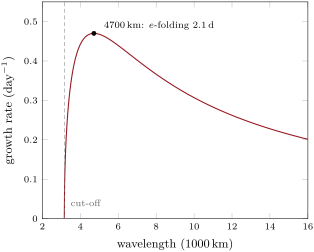
The growth rate depends only on the shear and the stratification, through $f\Lambda/N$, and the preferred size only on the Rossby radius. For the January mean at $45{}^{\circ}$ N the wind grows by $17.2\,\mathrm{m}/\mathrm{s}$ between $850\,\mathrm{hPa}$ and $250\,\mathrm{hPa}$, about $8.9\,\mathrm{km}$ apart in the standard atmosphere, a shear of $1.9 \times 10^{-3}\,\mathrm{s}^{-1}$; with the mean tropospheric $N = 0.0113\,\mathrm{s}^{-1}$ and $H = 11\,\mathrm{km}$, $L_d = 1210\,\mathrm{km}$, the fastest disturbance has a wavelength of $4700\,\mathrm{km}$ and grows by a factor $e$ in $2.1$ days. Disturbances shorter than $3200\,\mathrm{km}$ do not grow at all. These are the size and the growing time of the depressions on a weather map.

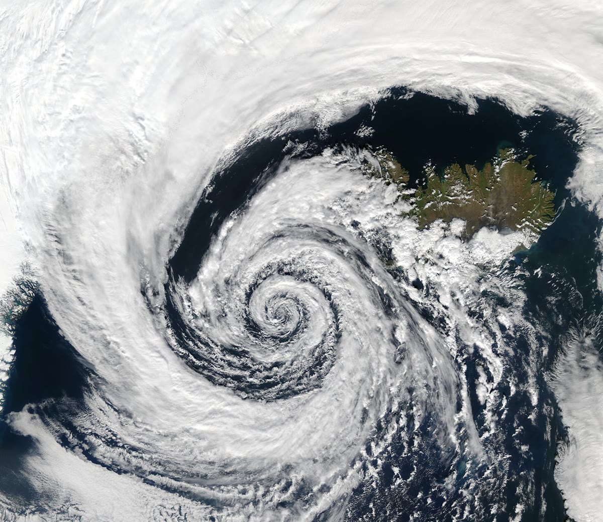
The extratropical cyclone of the Year 2 volume is the surface face of a growing baroclinic wave: its warm sector carries warm air poleward and upward, the cold air behind it slides equatorward and down, and the trough aloft tilts westward with height, as the release of available potential energy requires.

20.4 The general circulation

The general circulation is described by averaging round latitude circles, and what the average leaves out is as important as what it keeps.

Definition 20.11 (Zonal mean and eddies)

The zonal mean of a quantity $A$ is its average round a latitude circle at fixed height or pressure, $[A] = (1/2\pi)\int_0^{2\pi} A\,\mathrm d\lambda$. The departure $A^* = A - [A]$ is its eddy part; an eddy of the atmosphere is any departure of the flow from its zonal mean: travelling waves, stationary waves, cyclones and anticyclones.

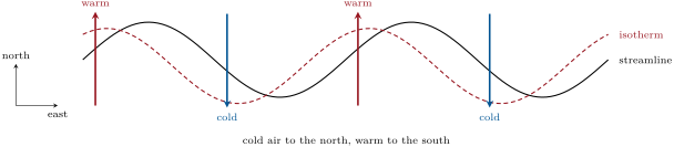
The zonal mean of a product splits in two: $[vT] = [v][T] + [v^*T^*]$. The first term is the transport by the mean meridional circulation, the cells of the Year 1 volume; the second the transport by the eddies. In the middle latitudes the mean meridional wind is weak and the eddy term dominates: poleward-moving air is warmer than equatorward-moving air at the same latitude, as in the figure below, and $[v^*T^*] > 0$. The eddies also carry westerly momentum, $[u^*v^*]$, from the subtropics into the latitudes of the jet, which is why the jet and the westerlies at the ground are maintained against friction. The Ferrel cell of the Year 1 volume is the mean meridional circulation that this eddy transport forces.

In the tropics the eddies are weak and the mean circulation carries heat poleward, the Hadley cell. The Year 1 volume found that air leaving the equator at rest and keeping its angular momentum would blow at hundreds of metres per second at $40{}^{\circ}$, and left open why the cell ends near $30{}^{\circ}$. A simple model answers.

Definition 20.12 (Atmospheric angular momentum; Held–Hou model)

The atmospheric angular momentum per unit mass about the Earth’s axis is $M = (\Omega a\cos\varphi + u)\,a\cos\varphi$, for an eastward wind $u$ at latitude $\varphi$. The Held–Hou model of the Hadley cell is an axisymmetric, steady circulation of a dry Boussinesq atmosphere of depth $H$, heated by relaxation towards a radiative-equilibrium potential temperature $\theta_E/\theta_0 = 1 + \Delta/3 - \Delta\sin^2\varphi$; its upper branch conserves $M$, its lower branch has negligible wind, and the flow is in thermal-wind balance.

Theorem 20.13 (Extent of the Hadley cell)

In the small-angle limit, the Held–Hou cell reaches the latitude

$$\varphi_H = \left(\frac{5\,gH\Delta}{3\,\Omega^2a^2}\right)^{1/2}$$

in each hemisphere, and the wind of its upper branch is $u_M = \Omega a\varphi^2$.

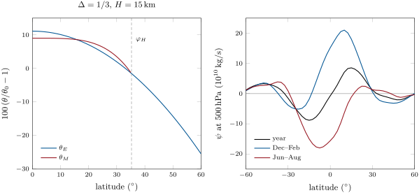
The cell ends where the temperature that angular-momentum conservation imposes meets radiative equilibrium; beyond, the atmosphere would have to be colder than radiation makes it. The model has two parameters that are not observed directly. For $H = 15\,\mathrm{km}$ and $\Delta$ between $1/6$ and $1/3$, chosen for illustration, $\varphi_H$ is $25{}^{\circ}$ to $35{}^{\circ}$. The observed cells, read from the zonal-mean meridional wind, end at $33.3{}^{\circ}$ N and $32.5{}^{\circ}$ S in the annual mean, and the winter cells, the strong ones, at $30.8{}^{\circ}$ N in December–February and $29.1{}^{\circ}$ S in June–August. The scaling is the point: a cell that widens with a deeper troposphere and a stronger heating contrast, and narrows on a faster-rotating planet. The model’s upper wind, $u_M = 88\,\mathrm{m}/\mathrm{s}$ at its edge for $\Delta = 1/6$, is twice the observed jet: the eddies take the excess away.

History — From long waves to the first computed forecast

In 1939 C.-G. Rossby and his collaborators, in the Journal of Marine Research, set out to interpret several apparently independent phenomena of the weather from a single point of view. Motivated by weather patterns that move upstream against the prevailing westerly flow, Rossby wrote down a linearised theory in which large-scale disturbances tend to move westward and smaller ones eastward relative to the wind: the waves and the $\beta$-plane of this chapter. Eleven years later J. G. Charney, R. Fjørtoft and J. von Neumann integrated the barotropic vorticity equation numerically on the electronic computer ENIAC: four forecasts of 24 hours at the $500\,\mathrm{mb}$ level, on a grid of $736\,\mathrm{km}$, 8 degrees of longitude at $45{}^{\circ}$. The computation of each forecast took about 24 hours: they were, as they wrote, just able to keep pace with the weather.

20.5 Exercises

Exercise 20.1 ★

(a) Compute the relative vorticity of a vortex in solid rotation that turns once a day. (b) Compute the planetary vorticity at $30{}^{\circ}$ and $60{}^{\circ}$ N ($\Omega = 7.292 \times 10^{-5}\,\mathrm{rad}/\mathrm{s}$) and compare.

Solution

Solution of Exercise 20.1.

(a) $\zeta = 2\omega = 2\times2\pi/86\,400 = 1.45 \times 10^{-4}\,\mathrm{s}^{-1}$. (b) $f = 7.29 \times 10^{-5}$ and $1.26 \times 10^{-4}\,\mathrm{s}^{-1}$: the vortex has about twice the planetary vorticity of $30{}^{\circ}$ N and a little more than that of $60{}^{\circ}$ N.

Exercise 20.2 ★

A parcel with no relative vorticity at $30{}^{\circ}$ N moves to $40{}^{\circ}$ N in a flow without divergence. Compute its relative vorticity there. Is it cyclonic or anticyclonic?

Solution

Solution of Exercise 20.2.

$\zeta = f_{30} - f_{40} = 7.29 \times 10^{-5} - 9.37 \times 10^{-5} = -2.08 \times 10^{-5}\,\mathrm{s}^{-1}$: anticyclonic.

Exercise 20.3 ★

At $45{}^{\circ}$ N, with no mean wind, compute the phase speed of a Rossby wave of wavelength $5000\,\mathrm{km}$ with $l = 0$. In which direction does it move?

Solution

Solution of Exercise 20.3.

$k = 2\pi/(5\times10^6) = 1.257 \times 10^{-6}\,\mathrm{m}^{-1}$; $c = -\beta/k^2 = -1.62 \times 10^{-11}/1.58 \times 10^{-12} = -10.3\,\mathrm{m}/\mathrm{s}$: westward.

Exercise 20.4 ★

At $60{}^{\circ}$ N in a westerly of $10\,\mathrm{m}/\mathrm{s}$, compute $\beta$, the stationary wavelength and the number of stationary waves round the latitude circle ($a = 6371\,\mathrm{km}$).

Solution

Solution of Exercise 20.4.

$\beta = 2\Omega\cos60{}^{\circ}/a = 1.14 \times 10^{-11}\,\mathrm{m}^{-1}\,\mathrm{s}^{-1}$; $\lambda_s = 2\pi\sqrt{10/1.14 \times 10^{-11}} = 5870\,\mathrm{km}$; the circle, $20\,015\,\mathrm{km}$, holds $n_s = 3.4$ waves.

Exercise 20.5 ★★

A column of air $10\,\mathrm{km}$ deep, without relative vorticity at $45{}^{\circ}$ N, crosses a mountain range that squeezes it to $8\,\mathrm{km}$, then a basin where it is $12\,\mathrm{km}$ deep. Assuming it stays near $45{}^{\circ}$ N, compute its relative vorticity over the range and over the basin. Where will depressions tend to form?

Solution

Solution of Exercise 20.5.

$q = f/h$ is conserved: over the range $\zeta = f(8/10) - f = -2.06 \times 10^{-5}\,\mathrm{s}^{-1}$, anticyclonic; over the basin $f(12/10) - f = +2.06 \times 10^{-5}\,\mathrm{s}^{-1}$, cyclonic. Where columns are stretched, in the lee of the range and over the basin, cyclonic vorticity is created: there depressions tend to form.

Exercise 20.6 ★★

For the wave with five crests round the $45{}^{\circ}$ N circle ($l = 0$) in a westerly of $15\,\mathrm{m}/\mathrm{s}$, compute the phase speed and the group velocity. How long does the wave’s energy take to travel $5000\,\mathrm{km}$ east, and how long the pattern?

Solution

Solution of Exercise 20.6.

$k = 5/(a\cos45{}^{\circ}) = 1.11 \times 10^{-6}\,\mathrm{m}^{-1}$, $\beta/k^2 = 13.1\,\mathrm{m}/\mathrm{s}$: $c = 1.9\,\mathrm{m}/\mathrm{s}$, $c_g = 28.1\,\mathrm{m}/\mathrm{s}$. The energy covers $5000\,\mathrm{km}$ in $2.1$ days, the pattern in $31$ days.

Exercise 20.7 ★★

At $45{}^{\circ}$ N in a westerly of $15\,\mathrm{m}/\mathrm{s}$, a wave is confined between latitudes so that $l = \pi/(6000\,\mathrm{km})$. (a) Compute its stationary zonal wavenumber and wavelength. (b) Show that no stationary wave exists for $l = \pi/(3000\,\mathrm{km})$.

Solution

Solution of Exercise 20.7.

(a) $k^2 = \beta/U - l^2 = 1.079 \times 10^{-12} - 2.74 \times 10^{-13} = 8.05 \times 10^{-13}\,\mathrm{m}^{-2}$, $k = 8.97 \times 10^{-7}\,\mathrm{m}^{-1}$: $\lambda = 7000\,\mathrm{km}$ and $n = 4.0$, fewer waves than with $l = 0$. (b) $l^2 = 1.097 \times 10^{-12} > \beta/U = 1.079 \times 10^{-12}$: $k^2$ would be negative.

Exercise 20.8 ★★

In an Eady model at $45{}^{\circ}$ N, $\Lambda = 2 \times 10^{-3}\,\mathrm{s}^{-1}$, $N = 0.012\,\mathrm{s}^{-1}$ and $H = 10\,\mathrm{km}$. Compute $L_d$, the growth rate and $e$-folding time of the fastest-growing disturbance, and its wavelength.

Solution

Solution of Exercise 20.8.

$L_d = 0.012\times10^4/1.031 \times 10^{-4} = 1164\,\mathrm{km}$; $\sigma = 0.31\times1.031 \times 10^{-4}\times2 \times 10^{-3}/0.012 = 5.3 \times 10^{-6}\,\mathrm{s}^{-1}$, an $e$-folding time of $2.2$ days; wavelength $2\pi\times1164/1.61 = 4540\,\mathrm{km}$.

Exercise 20.9 ★★

Along a latitude circle the eddy meridional wind is $v^* = V\cos kx$ and the eddy temperature $T^* = T_0\cos(kx - \delta)$, with $V = 10\,\mathrm{m}/\mathrm{s}$ and $T_0 = 5\,\mathrm{K}$. Compute $[v^*T^*]$ for $\delta = 0$, $60{}^{\circ}$ and $90{}^{\circ}$, and the corresponding heat flux $\rho c_p[v^*T^*]$ per $\mathrm{kg}/\mathrm{m}^{3}$ of air ($c_p = 1004\,\mathrm{J}\,\mathrm{kg}^{-1}\,\mathrm{K}^{-1}$). Which arrangement transports no heat?

Solution

Solution of Exercise 20.9.

$[v^*T^*] = (VT_0/2)\cos\delta$: $25\,\mathrm{K}\,\mathrm{m}/\mathrm{s}$, $12.5\,\mathrm{K}\,\mathrm{m}/\mathrm{s}$ and 0; heat fluxes $25\,100$, $12\,600$ and $0\,\mathrm{W}/\mathrm{m}^{2}$. When the temperature is a quarter wavelength out of phase with the wind, as much warm air goes south as north: no transport.

Exercise 20.10 ★★★

Starting from the barotropic vorticity equation, derive the dispersion relation of Rossby waves in a uniform westerly, and show that relative to the air every Rossby wave moves westward.

Solution

Solution of Exercise 20.10.

Linearising about $U$ with $\zeta' = \nabla^2\psi'$ and $v' = \partial_x\psi'$: $(\partial_t + U\partial_x)\nabla^2\psi' + \beta\partial_x \psi' = 0$. With $\psi' \propto \mathrm e^{\mathrm i(kx + ly - \omega t)}$, $(\omega - Uk)K^2 = -\beta k$, so $\omega = Uk - \beta k/K^2$. Relative to the air the phase speed is $c - U = -\beta/K^2 < 0$ for every wave.

Exercise 20.11 ★★★

In the Held–Hou model take $H = 12\,\mathrm{km}$ and $\Delta = 1/4$. Compute $\varphi_H$, the small-angle wind $u_M$ at the edge and the exact angular-momentum wind there, and compare with the subtropical jet of $44\,\mathrm{m}/\mathrm{s}$ of the January zonal mean.

Solution

Solution of Exercise 20.11.

$\varphi_H = [5\times9.81\times12\,000\times0.25/(3\times(7.292 \times 10^{-5})^2 \times(6.371 \times 10^{6})^2)]^{1/2} = 0.477\,\mathrm{rad}$, $27.3{}^{\circ}$. $u_M = \Omega a\varphi_H^2 = 106\,\mathrm{m}/\mathrm{s}$; exactly, $\Omega a\sin^2 \varphi_H/\cos\varphi_H = 110\,\mathrm{m}/\mathrm{s}$: two and a half times the observed jet.

Exercise 20.12 ★★★

Two layers of air differ in potential temperature by $10\,\mathrm{K}$ on $300\,\mathrm{K}$; their interface slopes upward towards the pole with slope $s$ across a band $4000\,\mathrm{km}$ wide, and $\rho = 0.7\,\mathrm{kg}/\mathrm{m}^{3}$. (a) Show that letting the interface flatten releases $\rho g' s^2L^2/24$ per unit area, $g' = g\,\Delta\theta/\theta$. (b) Compute it for $s = 10^{-3}$ and $2\times10^{-3}$ and compare with the kinetic energy of a $15\,\mathrm{m}/\mathrm{s}$ wind through $10\,\mathrm{km}$ of the same air.

Solution

Solution of Exercise 20.12.

(a) Across the band the interface is displaced by $\eta = sy$, $-L/2 \le y \le L/2$, from its flat position. A layer of reduced density contrast displaced by $\eta$ stores $\tfrac12\rho g'\eta^2$ per unit area; averaged over the band, $\langle\eta^2\rangle = s^2L^2/12$. (b) $g' = 0.327$: $1.5 \times 10^{5}$ and $6.1 \times 10^{5}\,\mathrm{J}/\mathrm{m}^{2}$, against $\tfrac12\times0.7\times15^2 \times10^4 = 7.9 \times 10^{5}\,\mathrm{J}/\mathrm{m}^{2}$ of kinetic energy: comparable.

20.6 Problem: The Wave that Stood Still

Problem 20.1

Weekend problem — vorticity, Rossby waves and the growth of a baroclinic wave at $45{}^{\circ}$ N

A westerly flow of $15\,\mathrm{m}/\mathrm{s}$ crosses the middle latitudes of an invented continent, along $45{}^{\circ}$ N. Take $\Omega = 7.292\,115 \times 10^{-5}\,\mathrm{rad}/\mathrm{s}$, $a = 6371\,\mathrm{km}$ and $g = 9.81\,\mathrm{m}/\mathrm{s}^{2}$. All values of the flow are invented.

Part I — A displaced parcel.

1. A parcel without relative vorticity at $45{}^{\circ}$ N is pushed to $50{}^{\circ}$ N. Compute $f$ at both latitudes and its relative vorticity at $50{}^{\circ}$ N, if the flow has no divergence.
2. Moving at $15\,\mathrm{m}/\mathrm{s}$, along what radius of curvature does it turn (take $\zeta = -V/R$, all of it from curvature)? Which way does it turn?
3. If its column also shrinks from $10.0\,\mathrm{km}$ to $9.5\,\mathrm{km}$ on the way, what is its relative vorticity at $50{}^{\circ}$ N?
4. Pushed instead to $40{}^{\circ}$ N, without divergence, what relative vorticity does it acquire? Explain why a parcel displaced from its latitude oscillates about it.

Part II — Travelling waves.

5. Compute $\beta$ at $45{}^{\circ}$ N and the length of the latitude circle.
6. For $n = 3$ to 8 waves round the circle ($l = 0$), compute the wavelength, the phase speed and the group velocity in the westerly of $15\,\mathrm{m}/\mathrm{s}$.
7. Which waves move west, which east? How many days does the wave $n = 5$ take to move $1000\,\mathrm{km}$?
8. A ridge over the west of the continent intensifies. Where, and after how long, will the effect of the wave $n = 6$ reach $5000\,\mathrm{km}$ downstream?

Part III — The wave that stood still.

9. Compute the stationary wavelength and the stationary wavenumber at $45{}^{\circ}$ N.
10. Compute the stationary wavenumber for westerlies of 10 and $20\,\mathrm{m}/\mathrm{s}$. What happens to the stationary waves when the westerlies strengthen in winter?
11. Compute the stationary wavenumber at $35{}^{\circ}$ N and $55{}^{\circ}$ N in the westerly of $15\,\mathrm{m}/\mathrm{s}$.
12. The continent’s western mountains rise $2\,\mathrm{km}$ into a troposphere $10\,\mathrm{km}$ deep. Compute the relative vorticity of a column that crosses them without changing latitude. Why do mountains force stationary waves?
13. Why does the wave pattern that the mountains force stand still only when its wavelength is near $\lambda_s$?

Part IV — A storm grows.

14. The westerly increases from the ground to $10\,\mathrm{km}$ by $25\,\mathrm{m}/\mathrm{s}$. Compute the shear $\Lambda$, and the poleward temperature gradient that it implies by the thermal wind at a mean temperature of $250\,\mathrm{K}$.
15. With $N = 0.011\,\mathrm{s}^{-1}$, compute the Richardson number $N^2/\Lambda^2$. Is the flow unstable to small-scale shear turbulence?
16. Compute the Rossby radius $L_d$ for $H = 10\,\mathrm{km}$.
17. Compute the wavelength of the fastest-growing Eady disturbance and the number of such waves round the latitude circle.
18. Compute the shortest wavelength that grows.
19. Compute the growth rate $\sigma_{\max}$.
20. By what factor does the disturbance grow in three days?
21. Compare the wavelength of the growing storm with the stationary wavelength of Part III: which is longer, and what does that imply for the motion of the storms relative to the stationary waves?
22. Which way does the trough of the growing wave tilt with height, and why must it?
23. Give the $e$-folding time of the fastest-growing Eady disturbance.

Solution

Solution of Problem 20.1.

1. $f_{45} = 1.031 \times 10^{-4}\,\mathrm{s}^{-1}$, $f_{50} = 1.117 \times 10^{-4}\,\mathrm{s}^{-1}$; $\zeta = f_{45} - f_{50} = -8.6 \times 10^{-6}\,\mathrm{s}^{-1}$.

2. $R = V/|\zeta| = 15/8.6 \times 10^{-6} = 1750\,\mathrm{km}$; clockwise, back towards the south.

3. $\zeta = f_{45}(9.5/10) - f_{50} = -1.38 \times 10^{-5}\,\mathrm{s}^{-1}$, more anticyclonic.

4. $\zeta = f_{45} - f_{40} = +9.4 \times 10^{-6}\,\mathrm{s}^{-1}$, cyclonic: it turns back north. Displaced either way, the parcel acquires the vorticity that turns it back: a restoring effect, and an oscillation.

5. $\beta = 1.62 \times 10^{-11}\,\mathrm{m}^{-1}\,\mathrm{s}^{-1}$; the circle is $28\,306\,\mathrm{km}$ long.

6. $n = 3$ to 8: wavelengths 9435, 7076, 5661, 4718, 4044 and $3538\,\mathrm{km}$; $c = -21.5$, $-5.5$, 1.9, 5.9, 8.3 and $9.9\,\mathrm{m}/\mathrm{s}$; $c_g = 51.5$, 35.5, 28.1, 24.1, 21.7 and $20.1\,\mathrm{m}/\mathrm{s}$.

7. $n = 3$ and 4 move west, $n \ge 5$ east. The wave $n = 5$ takes $10^6/1.86 = 5.4 \times 10^{5}\,\mathrm{s}$, $6.2$ days, to move $1000\,\mathrm{km}$.

8. Downstream, east: at $c_g = 24.1\,\mathrm{m}/\mathrm{s}$ the energy covers $5000\,\mathrm{km}$ in $2.4$ days.

9. $\lambda_s = 2\pi\sqrt{15/1.62 \times 10^{-11}} = 6050\,\mathrm{km}$, $n_s = 4.7$.

10. $n_s = 5.7$ for $10\,\mathrm{m}/\mathrm{s}$ and 4.1 for $20\,\mathrm{m}/\mathrm{s}$: a stronger westerly favours longer stationary waves, fewer round the hemisphere.

11. $n_s = 5.8$ at $35{}^{\circ}$ N and 3.4 at $55{}^{\circ}$ N.

12. $\zeta = f(8/10) - f = -2.06 \times 10^{-5}\,\mathrm{s}^{-1}$: squeezing over the mountains makes the column anticyclonic, stretching in the lee cyclonic. The mountains impose a fixed pattern of vorticity on the flow, a forcing that does not move.

13. A fixed forcing produces a steady response; the response is strongest when the forced pattern is itself a free wave that would stand still, the resonance at $\lambda_s$.

14. $\Lambda = 25/10^4 = 2.5 \times 10^{-3}\,\mathrm{s}^{-1}$; $|\partial T/\partial y| = \Lambda fT/g = 2.5 \times 10^{-3}\times1.031 \times 10^{-4} \times250/9.81 = 6.6\,\mathrm{K}$ per $1000\,\mathrm{km}$.

15. $\mathrm{Ri} = 0.011^2/(2.5 \times 10^{-3})^2 = 19$: far above 0.25, no shear turbulence.

16. $L_d = 0.011\times10^4/1.031 \times 10^{-4} = 1067\,\mathrm{km}$.

17. $2\pi\times1067/1.61 = 4160\,\mathrm{km}$; $28306/4160 = 6.8$ waves.

18. $2\pi\times1067/2.40 = 2790\,\mathrm{km}$.

19. $\sigma = 0.31\times1.031 \times 10^{-4}\times2.5 \times 10^{-3}/0.011 = 7.3 \times 10^{-6}\,\mathrm{s}^{-1}$, $0.63$ day$^{-1}$.

20. $\exp(3\times0.627) = 6.6$.

21. The storm, $4160\,\mathrm{km}$, is shorter than the stationary wavelength, $6050\,\mathrm{km}$: as a Rossby wave it is carried east by the westerly, and the storms travel east through the slower or standing long waves.

22. Westward with height: only then is the poleward-moving air warmer than the equatorward-moving air, so that heat goes poleward and the available potential energy is released.

23. The fastest-growing disturbance grows by a factor $e$ every $1.6$ days ($1.59$ days by the calculation).