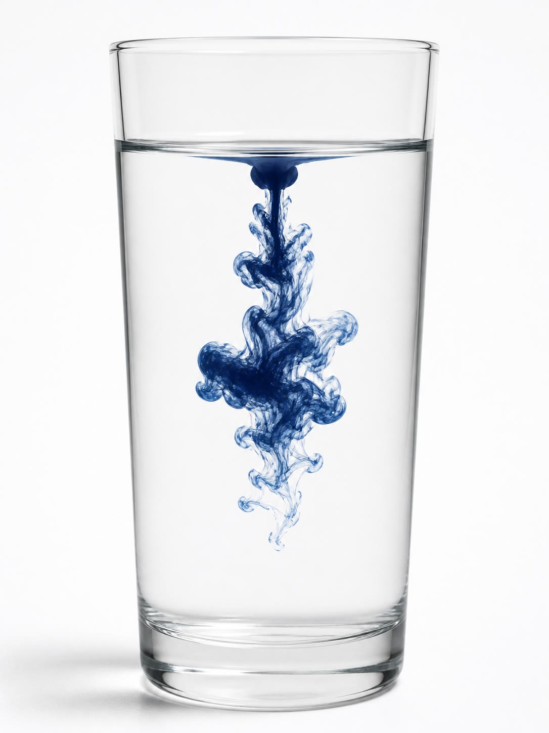
Drop a crystal of dye into still water and watch: a coloured cloud forms around it, grows, softens at its edges, and spreads — in a minute over a millimetre, in an hour over a centimetre, in a week over the glass. Nothing pushes the dye; it is carried by the ceaseless jostling of the molecules, which sends each particle on a random walk and, on average, from where there are many to where there are few. This is diffusion, the slowest and most universal of transports: it feeds every cell with oxygen, dopes every transistor with boron, hardens steel with carbon, and lets a perfume cross a room — though, as we shall see, not in the time one might think. This chapter gives diffusion its law (Fick), its equation (from a particle balance), its characteristic solutions and time scales (L∼Dt), and its microscopic origin in the random walk — which also explains why the diffusion equation, unlike every equation of mechanics, knows the direction of time. The next chapter will reuse all of it for heat.
Ink released in still water: the sharp cloud blurs and spreads as its molecules diffuse — over millimetres in a minute, centimetres in an hour.
24.1 Particle density, flux and Fick’s law
Definition 24.1(Density and particle current)
For a species of particles (molecules, ions, atoms in a solid) the number densityn(M,t) is the number of particles per unit volume around M (in m−3; the molar concentration is c=n/NA). The particle current densityjN is the vector such that the number of particles crossing an oriented surface element dS in dt is jN⋅dSdt (in m−2s−1): the particle flux through a surface S is ΦN=∬SjN⋅dS, the number of particles per second through S. For particles carried by a fluid moving at v, jN=nv (convection); diffusion is the transport that remains in a fluid at rest.
Theorem 24.2(Fick’s law)
In a medium at rest, where the density is not uniform, a particle current appears, proportional and opposite to the gradient of the density:
jN=−Dgradn,
where the diffusion coefficientD>0 (in m2/s) depends on the diffusing species, on the medium and on the temperature. Particles go down the density gradient, from the denser to the rarer regions, at a rate set by D.
Proof. Phenomenological (a law of experience, like Ohm’s): linear in the gradient for small gradients, isotropic in an isotropic medium, and with the sign that experience imposes. The random-walk model of Section 24.4 derives it, and D with it, from the molecular motion. ∎
Example 24.3(Orders of magnitude of D)
Gases: D∼1×10⁻⁵m2/s (water vapour in air 2.5×10⁻⁵m2/s, a perfume molecule 5×10⁻⁶m2/s). Liquids: D∼1×10⁻⁹m2/s (oxygen in water 2×10⁻⁹m2/s, sugar 5×10⁻¹⁰m2/s, a protein 1×10⁻¹⁰m2/s). Solids: tiny and steeply increasing with temperature, D=D0e−Ea/kBT (boron in silicon: 1.5×10⁻¹⁷m2/s at 1100∘C, unmeasurably small at room temperature — which is why a transistor, once made, keeps its doping profile for decades). Four orders of magnitude from gas to liquid, eight or more from liquid to solid.
24.2 The particle balance and the diffusion equation
Theorem 24.4(Local particle balance)
If the particles are neither created nor destroyed,
∂t∂n+divjN=0;
with a source creating σ particles per unit volume and time (a chemical reaction, an absorption), ∂tn+divjN=σ. In one dimension (density and current depending on x only): ∂tn+∂xjN=0.
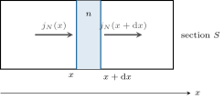
Proof. Take the slab between x and x+dx, of section S: it holds nSdx particles; in dt, jN(x)Sdt enter through the left face and jN(x+dx)Sdt leave through the right one, so ∂tnSdxdt=−(jN(x+dx)−jN(x))Sdt=−∂xjNdxSdt. In three dimensions the same count on a small box gives the divergence (the flux out of a closed surface per unit volume, Chapter 11), or directly: for any fixed volume V, d/dt∭Vndτ=−∬∂VjN⋅dS=−∭VdivjNdτ by the Ostrogradski theorem. ∎
The one-dimensional balance: the slab between x and x+dx gains what enters on the left and loses what leaves on the right; the difference is the change of n inside.
Theorem 24.5(Diffusion equation)
Combining Fick’s law and the balance, for uniform D,
∂t∂n=DΔn+σ,in one dimension∂t∂n=D∂x2∂2n+σ.
This diffusion equation is linear (solutions superpose), first order in time and second order in space — not a wave equation: it has no propagation speed, but a characteristic relation between length and time,
L∼Dt,t∼DL2:
diffusing over twice the distance takes four times as long.
Proof.∂tn=−div(−Dgradn)+σ=Ddivgradn+σ=DΔn+σ. For the scales, compare n/t with Dn/L2. ∎
Remark 24.6(Diffusion is irreversible)
Change t into −t in the wave equation, ∂t2u=c2∂x2u, and it is unchanged: a film of a wave run backwards is a possible wave. Do the same in the diffusion equation and the sign of the left side flips: n(x,−t) is not a solution. A cloud that spreads is natural; a cloud that spontaneously gathers into a crystal is not — diffusion has an arrow of time, the arrow of the second law (Chapter 25 computes the entropy it creates). The equation also shows that diffusion smooths: where n is locally a maximum (∂x2n<0) it decreases, where it is a minimum it increases.
Example 24.7(How long does it take?)
t∼L2/D. Oxygen across a cell, L=10µm in water: 10−10/2×10−9=0.05s — diffusion feeds a cell with ease; across 1mm of tissue: 500s — too slow, which is why nothing living is thicker than a fraction of a millimetre without blood vessels. Sugar across a cup of unstirred tea, L=5cm: 2.5×10⁻³/5×10−10=5×106s, two months — stir. A perfume across a room by diffusion alone, 5m in air: 25/10−5=3×106s, a month; you smell it within a minute because the air moves: convection carries, diffusion only completes the last millimetres.
24.3 Characteristic solutions
Proposition 24.8(Stationary regime: the membrane)
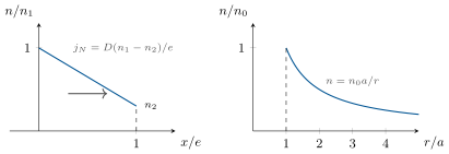
Between two reservoirs held at n1 and n2, across a membrane of thickness e and area S, the stationary density is linear,
the membrane has a diffusive resistancee/DS, exactly as a wire has ℓ/γS — resistances in series add, and a thin membrane of small D can still dominate.
Proof. Stationary, one-dimensional, no source: ∂x2n=0, so n is affine; jN=−Ddn/dx is uniform. ∎
Around a sphere of radius a whose surface is held at n0, in a medium where n→0 far away, the stationary density is
n(r)=n0ra,ΦN=4πDan0:
the total current released (or absorbed, with the signs reversed) grows with the radius, not the surface, of the sphere — the geometry of a diffusive sink is that of an electrostatic capacitance.
Proof.Δn=r21drd(r2dn/dr)=0 gives n=A+B/r; the boundary conditions fix A=0, B=n0a; then ΦN=−4πr2Ddn/dr=4πDn0a at every r (no accumulation in the stationary regime). ∎
Stationary profiles. Left: across a membrane the density is linear and the current uniform. Right: around a sphere the density falls as 1/r; the total current 4πDan0 is proportional to the radius.
Proposition 24.10(The spreading Gaussian)
N particles per unit area released at t=0 on the plane x=0 of an infinite medium spread as
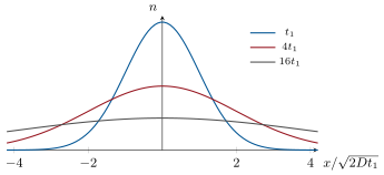
n(x,t)=4πDtNexp(−4Dtx2):
a Gaussian of standard deviation σ(t)=2Dt, of constant area N (the particles are conserved) and decreasing peak ∝1/t. In three dimensions, N particles released at a point spread as n=N(4πDt)−3/2exp(−r2/4Dt), with ⟨r2⟩=6Dt. A pulse of particles released at the surface of a half-space (which they cannot leave) gives twice the expression above for x>0.
Proof. Substitute: with u=x2/4Dt, ∂tn=n(−1/2t+u/t) and D∂x2n=Dn(−1/2Dt+x2/4D2t2)=n(−1/2t+u/t); equal. The normalisation ∫ndx=N follows from ∫e−x2/4Dtdx=4πDt, and ∫x2ndx/N=2Dt. Uniqueness (given the initial pulse) is admitted. ∎
The Gaussian solution at three times: the width grows as t, the peak falls as 1/t, the area (the number of particles) stays the same.
Proposition 24.11(Constant surface concentration)
A half-space x>0 initially empty, whose surface is held at the density n0 from t=0 (a gas in contact with a solid that dissolves it), fills as
n(x,t)=n0erfc(2Dtx),erfc(u)=π2∫u∞e−s2ds,
the complementary error function, which falls from 1 at u=0 to 0.16 at u=1 and 0.005 at u=2: the penetration depth is again ∼2Dt, and the total number of particles absorbed per unit area is 2n0Dt/π.
Proof. Look for n=f(u) with u=x/2Dt: the equation becomes f′′+2uf′=0, so f′∝e−u2 and f is an error function; the conditions f(0)=n0, f(∞)=0 select erfc. The absorbed number is ∫0∞ndx=n02Dt∫0∞erfc(u)du=2n0Dt/π. ∎
Example 24.12(Hardening steel)
A steel part held at 900∘C in a carbon-rich gas absorbs carbon at its surface; with D=5×10⁻¹²m2/s for carbon in hot iron, four hours give 2Dt=0.5mm: a hard skin of half a millimetre on a tough core — the case hardening of gears and bearings, timed with the erfc profile.
24.4 The microscopic picture: random walk
Proposition 24.13(Random walk and the diffusion coefficient)
A particle that makes a step of length ℓ in a random direction every τ (a molecule between two collisions) has, after N=t/τ steps, a mean square displacement
D=2τℓ2(1D),D=6τℓ2=6ℓv∗∼3ℓv∗(3D, with v∗=ℓ/τ; the kinetic theory gives 31).
The walker’s distance grows as t, not t: to go twice as far it needs four times as many steps.
Proof.x=∑iϵiℓ with independent ϵi=±1 (1D): ⟨x2⟩=∑i,j⟨ϵiϵj⟩ℓ2=Nℓ2, the cross terms averaging to zero. The distribution of x for large N tends to a Gaussian (the central limit theorem, whose proof belongs to the probability course) — which is why the macroscopic law is the diffusion equation; Fick’s law itself follows from counting the walkers crossing a plane from both sides: jN≈−21ℓv∗∂xn (a more careful average gives 1/3 in three dimensions). ∎
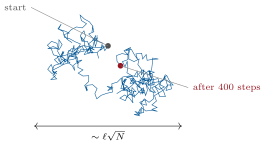
A random walk of 400 steps of length ℓ: the walker has wandered only some 20ℓ from its start — the N law that makes diffusion so slow over long distances and so fast over short ones.
Example 24.14(From molecules to D)
Air at room temperature: mean free path ℓ≈70nm, mean speed v∗≈500m/s: D≈ℓv∗/3=1.2×10−5m2/s, as measured. To diffuse 1m a molecule needs N=(L/ℓ)2=2×1014 collisions, i.e. Nℓ/v∗≈3×104s — eight hours for a trip it would make in 2ms if it flew straight. In a liquid, a sphere of radius a buffeted by the molecules obeys the Stokes–Einstein relation D=kBT/6πηa (Einstein 1905): for sugar, a≈0.4nm in water, D=5×10⁻¹⁰m2/s; for a 1µm grain, 4×10⁻¹³m2/s, a displacement of a micrometre per second — the Brownian motion that Perrin measured to count Avogadro’s number. In a solid an atom jumps to a neighbouring site only when a thermal fluctuation supplies the activation energy: D=D0e−Ea/kBT, doubling every few tens of kelvins near 1000∘C.
Method 24.15(Diffusion estimates)
(1) Identify D (gas 10−5, liquid 10−9, solid Arrhenius). (2) Time or distance: t∼L2/D, L∼Dt (with the exact 2Dt for the Gaussian width, 2Dt for the erfc depth). (3) Stationary: linear in a slab (Rd=e/DS), 1/r around a sphere (Φ=4πDaΔn), lnr around a cylinder. (4) Transient: Gaussian for a pulse, erfc for a held surface; superpose. (5) Ask whether convection does not dominate. (6) Microscopic check: D∼ℓv∗/3.
24.5 Exercises
Exercise 24.1★
Diffusion times L2/D: a sugar cube at the bottom of a 5cm cup (D=5×10⁻¹⁰m2/s); perfume across a 5m room (D=5×10⁻⁶m2/s); oxygen across 1mm of tissue and across a 10µm cell (D=2×10⁻⁹m2/s). Which of these does diffusion actually do?
Solution
Solution of Exercise 24.1.
L2/D: sugar 5×10⁶s (two months); perfume the same; tissue 500s; cell 0.05s. Diffusion really does the last one (and, barely, the second to last); convection does the rest.
Exercise 24.2★
A membrane 1µm thick and 1cm2 in area, D=1×10⁻¹¹m2/s inside it, separates a solution at 1mol/m3 from pure water. Current density, molar flux and number of molecules per second; diffusive resistance; with two such membranes in series.
Solution
Solution of Exercise 24.2.
j=DΔn/e=1×10−5mol/m2/s; ×1×10⁻⁴m2: 1×10⁻⁹mol/s, 6×10¹⁴ molecules per second; Rd=e/DS=1×109s/m3; two in series: half.
Exercise 24.3★
A thin layer of dye (N=1×10²⁰m−2) is released in water, D=1×10⁻⁹m2/s. Width 2Dt and peak density after 1s, 1h, 1day. When has the peak fallen to 1% of its value at 1s?
Solution
Solution of Exercise 24.3.
2Dt: 45µm, 2.7mm, 13mm; peak N/4πDt: 9×10²³m−3, 1.5×10²²m−3, 3×10²¹m−3; 1% after 104 times longer: 1×10⁴s.
Exercise 24.4★
Air molecules: ℓ=70nm, v∗=500m/s. Estimate D; number of collisions and time to diffuse 1m; compare with the straight flight. Same for a molecule in water (ℓ≈0.1nm, v∗≈500m/s): is the estimate right, and why not exactly?
Solution
Solution of Exercise 24.4.
D≈1.2×10⁻⁵m2/s; N=(L/ℓ)2=2×1014; Nℓ/v∗=3×104s against 2ms. Water: the estimate gives 2×10⁻⁸m2/s, ten times the measured values — in a liquid a molecule rattles in the cage of its neighbours and its successive steps are anti-correlated; the effective step is shorter.
Exercise 24.5★★
Oxygen in a tissue. A slab of tissue of thickness 2a consumes oxygen at the uniform rate q (per unit volume); its two faces are held at n0. (a) Write the stationary equation with the sink and solve it. (b) Condition for oxygen to reach the centre. (c) D=2×10⁻⁹m2/s, n0=0.2mol/m3, q=0.01mol/m3/s: maximum a. (d) Conclude on the spacing of capillaries.
Solution
Solution of Exercise 24.5.
(a) Dn′′=q: n=n0−q(a2−x2)/2D. (b) n(0)≥0: a≤2Dn0/q. (c) 0.28mm. (d) No cell can be farther than a few hundred micrometres from a capillary (in practice 50–100µm in active tissue).
Exercise 24.6★★
A dissolving grain. A sugar sphere of radius a=1mm in still water keeps its surface at the saturation density ns=5800mol/m3; far away the water is pure; D=5×10⁻¹⁰m2/s. (a) Stationary profile and total current. (b) Number of moles in the grain (density 1590kg/m3, molar mass 342g/mol) and dissolution time (take the current constant). (c) Why is the true time longer, and why does stirring help so much? (d) Show that for a very long cylinder the stationary profile is logarithmic and the problem has no solution in an infinite medium.
Solution
Solution of Exercise 24.6.
(a) n=nsa/r, Φ=4πDans=3.6×10⁻⁸mol/s. (b) 1.95×10⁻⁵mol; 540s. (c) The 1/r shell takes ∼a2/D≈2000s to build and the grain shrinks; stirring replaces the shell of thickness ∼a by a boundary layerδ≪a and multiplies the flux by a/δ. (d) (rn′)′=0: n=A+Blnr, which cannot vanish at infinity: no stationary state — the cloud of a cylinder keeps growing (logarithmically).
Exercise 24.7★★
Conservation and irreversibility. (a) From the equation, show that ∫ndx is constant and that d⟨x2⟩/dt=2D (integrate by parts, n→0 at infinity). (b) Show that n(x,−t) does not satisfy the equation. (c) What becomes of the Gaussian solution for t<0? (d) Show that ∫n2dx can only decrease: diffusion flattens.
Solution
Solution of Exercise 24.7.
(a) d/dt∫n=D[n′]−∞∞=0; d/dt∫x2n=D∫x2n′′=2D∫n=2DN. (b) ∂t[n(x,−t)]=−D∂x2n: the sign flips. (c) For t<0 the “width” 2Dt is negative: no such state — the pulse cannot be unspread. (d) d/dt∫n2=2D∫nn′′=−2D∫n′2≤0.
Exercise 24.8★★
Carburising. Carbon in hot iron, D=5×10⁻¹²m2/s at 900∘C; surface held at n0. (a) Check that n0erfc(x/2Dt) solves the equation. (b) Depth at which n=0.1n0 after 4h (erfc(1.16)=0.1). (c) Time for twice the depth. (d) At 950∘C, D is 2.5 times larger: time saved.
Stokes–Einstein.D=kBT/6πηa, water η=1×10⁻³Pas, 300K. (a) D for a=1µm and the root-mean-square displacement in 1s, 1min. (b) D for a protein, a=3nm. (c) Sugar has D=5×10⁻¹⁰m2/s: effective radius. (d) How does measuring ⟨x2⟩ of a grain under a microscope give Avogadro’s number?
Solution
Solution of Exercise 24.9.
(a) D=2.2×10⁻¹³m2/s; 2Dt: 0.66µm, 5µm. (b) 7×10⁻¹¹m2/s. (c) a=kBT/6πηD=0.44nm. (d) ⟨x2⟩=2Dt=RTt/3πηaNA: every quantity but NA is measured.
Exercise 24.10★★★
Time lag of a membrane. A membrane of thickness e, initially empty, is exposed on one face to n1 at t=0, the other face kept at 0. (a) What is the final stationary flux? (b) Argue that the flux on the far face rises over a time ∼e2/D (the exact lag is e2/6D). (c) A drug patch with e=20µm, D=1×10⁻¹³m2/s through the skin’s outer layer: lag time. (d) Why is the lag useful to measure D and the stationary flux to measure D× solubility?
Solution
Solution of Exercise 24.10.
(a) Dn1S/e. (b) The particles need ∼e2/D to cross. (c) e2/6D=670s, eleven minutes. (d) The lag gives D alone; the stationary flux gives D× (solubility): two measurements, two unknowns.
Exercise 24.11★★★
The perfect absorber. A sphere of radius a absorbs every particle that touches it, in a medium at n∞ far away. (a) Stationary profile and total current captured. (b) A bacterium, a=1µm, in a sugar solution at n∞=6×10²⁰m−3, D=5×10⁻¹⁰m2/s: molecules captured per second. (c) Its surface is covered by Nr small absorbing receptors of radius s, the rest reflecting: each receptor alone captures ≈4Dsn∞ (a disc); show that the whole cell captures nearly the maximum once Nrs≫a, i.e. with a tiny fraction of its surface covered. (d) Comment: why cells can afford thousands of different receptors.
Solution
Solution of Exercise 24.11.
(a) n=n∞(1−a/r), Φ=4πDan∞. (b) 3.8×10⁶ per second. (c) Receptors act like conductances in parallel and then in series with the spherical shell: Φ≈4πDan∞⋅Nrs/(Nrs+πa); half the maximum for Nrs=πa: with s=1nm, Nr≈3000, covering Nrs2/4a2≈10−3 of the surface. (d) Each kind of receptor needs a negligible area for near-maximal capture: a cell can watch thousands of substances at once.
Exercise 24.12★★★
Solving it on a grid. Divide space into cells of size Δx and time into steps Δt; write nik+1=nik+α(ni+1k−2nik+ni−1k) with α=DΔt/Δx2. (a) Justify it from the equation. (b) Interpret it as a random walk when α=1/2. (c) Show that for α>1/2 a density alternating +,−,+,− from cell to cell grows: instability. (d) For the boron profile of the problem below (D=1.5×10⁻¹⁷m2/s, Δx=10nm), the largest stable Δt and the number of steps for one hour.
Solution
Solution of Exercise 24.12.
(a) Forward difference in t, centred second difference in x. (b) α=1/2: nik+1=(ni−1k+ni+1k)/2 — every particle hops left or right with probability 1/2. (c) For ni=(−1)i, nk+1=(1−4α)nk: ∣1−4α∣>1 when α>1/2. (d) Δt≤Δx2/2D=3.3s; about 1100 steps.
24.6 Problem: A doped wafer and a scented room
Problem 24.1
Weekend problem — diffusion in a solid and in a gas
Part I — Drive-in of boron in silicon. Boron diffuses in silicon with D=D0e−Ea/kBT, D0=7.6×10⁻⁵m2/s, Ea=3.46eV; kB=8.62×10⁻⁵eV/K. A dose Q=1×10¹⁸m−2 of boron has been deposited in a very thin layer at the surface of a wafer whose background doping is nB=1×10²¹m−3; it is then heated (“driven in”) at 1100∘C for one hour. The surface reflects the boron (no escape).
Compute D at 1100∘C and at 1000∘C. By what factor does it change over these 100K?
Why is the profile after the drive-in n(x,t)=(Q/πDt)exp(−x2/4Dt) and not the Gaussian of Proposition 24.10? Check that its integral over x>0 is Q.
Surface concentration after one hour.
The junction depthxj is where n=nB: compute it.
How does xj change if the drive-in lasts four hours? (Careful: the surface concentration changes too.)
Relative change of D for a 10K error in temperature; temperature control needed for xj to 1%.
At room temperature, D: estimate the time for the profile to move by one atomic spacing, and conclude.
Part II — Predeposition. The dose itself was put in at 950∘C from a gas that holds the surface at the solubility limit n0=2×1026m−3 for 30min.
D at 950∘C and Dt for 30min.
Profile at the end of the predeposition; depth at which n=nB (erfc(3.2)≈6×10⁻⁶).
Dose introduced; compare with the Q of Part I.
Why does one predeposit at a lower temperature and drive in at a higher one?
Justify that during the drive-in the predeposited layer can be treated as infinitely thin.
Part III — A perfume in a room. A drop of perfume (1mg, molar mass 150g/mol) evaporates at once in the corner of a still room at 300K, 1bar. Take the perfume molecule’s collision diameter with air as d=0.5nm and the number density of air na=P/kBT.
Mean free path ℓ=1/(2πd2na) of the perfume molecule, and its mean speed v∗=8RT/πM.
Estimate D=ℓv∗/3.
Time to diffuse 5m; and if the air drifts at 0.1m/s?
Write the three-dimensional Gaussian for the cloud (a corner: the walls reflect, multiply by 8). At a point 1m away, at what time is the concentration maximal?
Maximum number density there; compare with a perception threshold of 1×10¹³m−3.
The cloud’s edge: at what distance is the density 10−6 of its central value after one day?
Number of collisions a perfume molecule suffers in a day.
Part IV — The walker and the arrow of time.
A walker makes N steps ±ℓ on a line: mean and mean square displacement; show that ⟨x2⟩=2Dt identifies D=ℓ2/2τ.
Probability that the walker returns exactly to its start after N=2, 4, 6 steps; comment on the trend.
Film a diffusing cloud and run the film backwards: what do you see, and which equation is violated?
Explain in one paragraph how the reversible motion of molecules produces the irreversible diffusion equation.
Summarise: the length scale, the time scale, and the one quantity that distinguishes a gas, a liquid and a hot solid.
Solution
Solution of Problem 24.1.
1.kBT=0.118eV, Ea/kBT=29.2: D=1.6×10⁻¹⁷m2/s; at 1000∘C: 1.6×10⁻¹⁸m2/s — a factor 10.
2. The reflecting surface is handled by the mirror image of the pulse, doubling the amplitude on x>0; ∫0∞=(Q/πDt)⋅214πDt=Q.
3.Dt=5.8×10⁻¹⁴m2; πDt=0.43µm; ns=2.3×1024m−3.
4.e−x2/4Dt=4.3×10−4: xj2=4Dt×7.75, xj=1.3µm.
5.ns halves, the logarithm drops to 7.05, 4Dt quadruples: xj=2.6µm — less than doubled.
6.δD/D=(Ea/kBT)δT/T=21%; xj∝Dt roughly, so 1% on xj needs 2% on D: 1K.
7.Ea/kBT=134: D≈10−62m2/s; one spacing (0.25nm) in a2/D∼1043s: frozen.
10.2n0Dt/π=6.3×1018m−2: six times Q — the dose grows as t and is set by the time.
11. Low temperature: small D, dose controlled by time, shallow; high temperature: the fixed dose is driven deep quickly.
12.0.18µm against 1.3µm: thin.
13.4×10¹⁸ molecules; na=2.4×1025m−3.
14.ℓ=37nm; v∗=206m/s.
15.D≈2.5×10⁻⁶m2/s.
16.L2/D=107s, months; drifting: 50s.
17.n=8N(4πDt)−3/2e−r2/4Dt; maximal at t∗=r2/6D=6.7×104s, eighteen hours.
18.nmax=8N(4πDt∗)−3/2e−3/2≈2×1018m−3, far above threshold: smelt, eventually.
19.r2=4Dtln106=12m2: 3.5m.
20.v∗t/ℓ≈5×1014.
21.⟨x⟩=0, ⟨x2⟩=Nℓ2=ℓ2t/τ; D=ℓ2/2τ.
22.(N/2N)/2N: 1/2, 3/8, 5/16 — decreasing (as 1/πN/2): the walker wanders off as N.
23. The cloud gathers itself into a point — never seen; it violates the diffusion equation, not the laws of mechanics.
24. Each collision is reversible, but the initial state (all particles together) is exceptional: almost every microscopic history from it spreads, and the reverse needs a conspiracy of all the velocities. The random-walk average keeps only what is typical and discards that information; irreversibility is statistical.
25.L∼Dt, t∼L2/D; D∼ℓv∗/3, i.e. the step between collisions: 10−5, 10−9, 10−17m2/s.