University Physics — Year 2 · Bachelor Year 2

30The Schrödinger Equation and Wave Functions

Fire electrons one at a time at a pair of slits and record where each lands: a dot here, a dot there, apparently at random — and after ten thousand dots, the fringes of Young’s experiment, as if each electron had passed through both slits and interfered with itself. The last chapter of the Year 1 volume met this strangeness: light comes in photons, matter has a wavelength $\lambda = h/p$ , and position and momentum cannot both be sharp. What it did not give is the equation — the rule that says how the wave associated with a particle evolves, as Newton’s law says how a trajectory evolves. That equation is Schrödinger’s (1926), and with it the quantum description becomes a calculable theory: one writes a wave function $\psi(x,t)$ , whose squared modulus is the probability of finding the particle, and one solves a linear partial differential equation. This chapter states the equation, explains what $\psi$ means and what it does not, finds its stationary states and the free particle’s wave packets, and shows where Newton’s mechanics re-emerges — for everything heavier than a molecule.

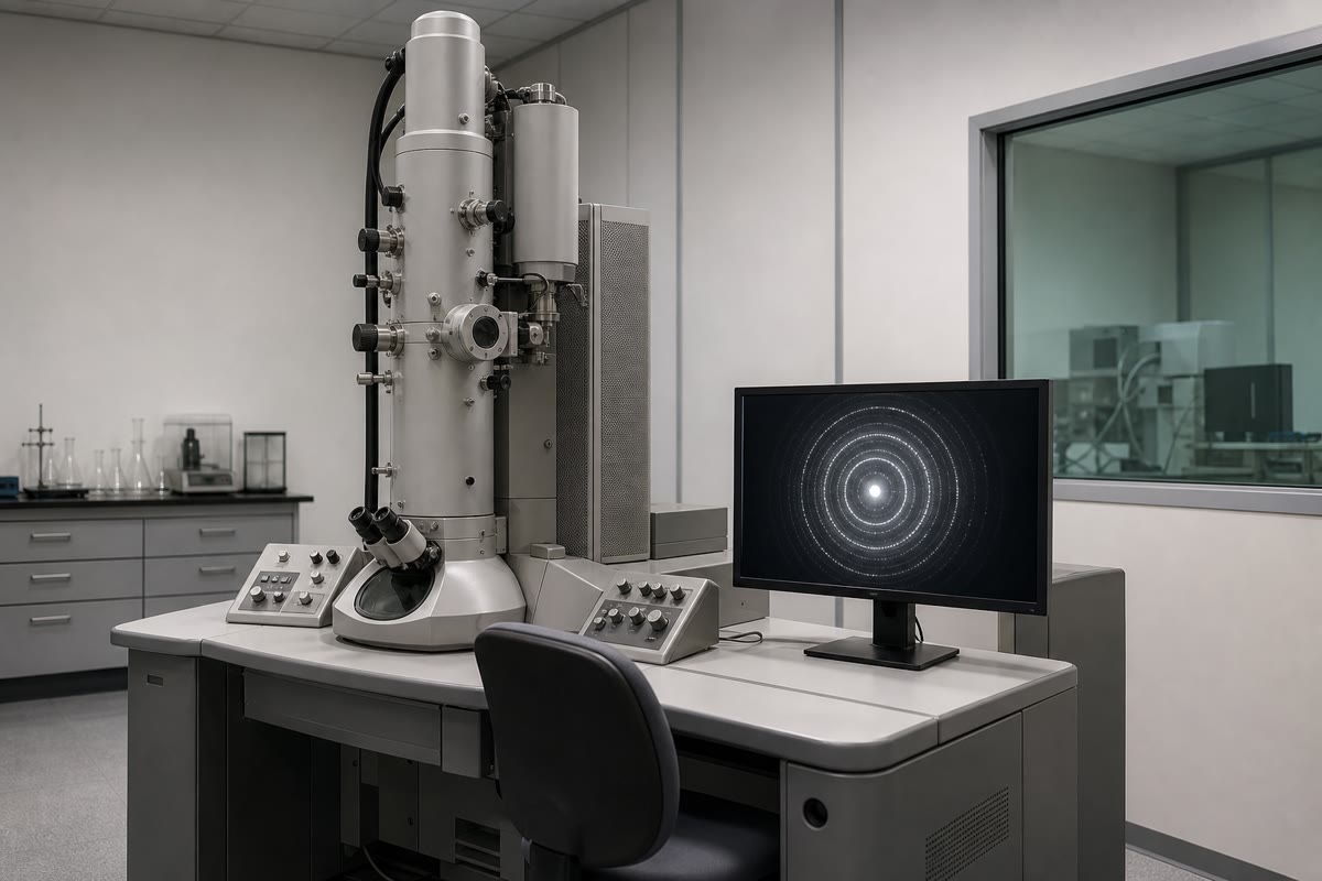
A transmission electron microscope: electrons accelerated to a hundred kilovolts have a wavelength of a few picometres, and their wave function, focused by magnetic lenses, images the atoms of a crystal.

30.1 What the Year 1 volume left us

Proposition 30.1 (Particles are waves)

A photon of frequency $\nu$ has the energy $E = h\nu = \hbar\omega$ and the momentum $p = h/\lambda = \hbar k$ ; a material particle of momentum $p$ behaves as a wave of wavelength $\lambda = h/p$ (de Broglie), with $E = \hbar\omega$ and $p = \hbar k$ as well — electron diffraction by crystals, neutron and even molecule interferometry confirm it; and no state can have a position and a momentum sharper than $\Delta x\,\Delta p \ge \hbar/2$ (Heisenberg). With $\hbar = h/2\pi = 1.05 \times 10^{-34}\,\mathrm{J}\,\mathrm{s}$ : an electron at $100\,\mathrm{eV}$ has $\lambda = 0.12\,\mathrm{nm}$ , the size of an atom; a dust grain of $1 \times 10^{-15}\,\mathrm{kg}$ at $1\,\mathrm{mm}/\mathrm{s}$ has $\lambda = 7 \times 10^{-16}\,\mathrm{m}$ , smaller than a nucleus — it behaves classically.

Proof. Recalled from the Year 1 volume; the task now is the dynamics of the wave. ∎

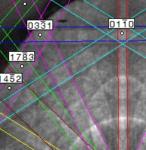
An electron diffraction pattern recorded in an electron microscope (a Kikuchi pattern from a crystal): electrons of a few picometres’ wavelength, diffracted by the atomic planes — matter behaving as a wave (NIST).

30.2 The wave function

Definition 30.2 (Wave function and Born’s rule)

The state of a particle moving along $x$ is described by a complex wave function $\psi(x,t)$ such that

\dd\mathcal P = |\psi(x,t)|^2\,\dd x

is the probability of finding the particle between $x$ and $x + \dd x$ at the time $t$ (Born’s rule); hence the normalisation $\int_{-\infty}^{\infty}|\psi|^2\dd x = 1$ , and the expectation values $\langle x\rangle = \int x|\psi|^2\dd x$ , $\Delta x^2 = \langle x^2\rangle - \langle x\rangle^2$ . Wave functions obey the superposition principle: if $\psi_1$ and $\psi_2$ are possible states, so is $\alpha\psi_1 + \beta\psi_2$ (normalised), and the probabilities then contain the interference term $2\operatorname{Re}(\alpha^*\beta\,\psi_1^*\psi_2)$ . A global phase factor $\eu^{\iu\theta}$ changes nothing; a relative phase between two superposed components changes the interference.

Remark 30.3 (What $\psi$ is not)

$\psi$ is not a classical field spread in space like $\vect E$ , nor a cloud of matter: the electron is always found whole, at one point. $\psi$ is an amplitude of probability, the object that interferes; only $|\psi|^2$ is observed, and only statistically, by repeating the experiment on identically prepared particles. The dots of the double slit are single electrons; the fringes are $|\psi_1 + \psi_2|^2$ .

30.3 The Schrödinger equation

Theorem 30.4 (Schrödinger equation)

A particle of mass $m$ in the potential energy $V(x)$ has a wave function obeying

\iu\hbar\,\frac{\partial\psi}{\partial t} = -\frac{\hbar^2}{2m}\,\frac{\partial^2\psi}{\partial x^2} + V(x)\,\psi .

It is linear (superposition), first order in time (the wave function at one instant determines it at all later times), and complex ( $\psi$ cannot be real: the $\iu$ is essential). It is a postulate, justified by its consequences.

Proof. A motivation rather than a proof. A free particle of sharp momentum $p = \hbar k$ and energy $E = \hbar\omega$ should be a plane wave $\psi = A\eu^{\iu(kx - \omega t)}$ , for which $\iu\hbar\partial_t\psi = \hbar\omega\psi = E\psi$ and $-(\hbar^2/2m)\partial_x^2\psi = (\hbar^2k^2/2m)\psi = (p^2/2m)\psi$ . The classical relation $E = p^2/2m$ is thus reproduced by the equation $\iu\hbar\partial_t\psi = -(\hbar^2/2m)\partial_x^2\psi$ , and the natural generalisation for $E = p^2/2m + V$ adds $V\psi$ . Notice that the equation must be linear to hold for superpositions of plane waves, and first order in time with an $\iu$ so that $\eu^{-\iu\omega t}$ and not $\cos\omega t$ is the time dependence — a real wave equation would give $E^2 \propto p^4$ . ∎

Proposition 30.5 (Conservation of probability)

The probability density $\rho = |\psi|^2$ and the probability current

j = \frac{\hbar}{m}\operatorname{Im}\Big(\psi^*\frac{\partial\psi}{\partial x}\Big) = \frac{\hbar}{2\iu m}\Big(\psi^*\partial_x\psi - \psi\,\partial_x\psi^*\Big)

obey $\partial_t\rho + \partial_xj = 0$ : probability is neither created nor destroyed, and $\int|\psi|^2\dd x$ stays equal to $1$ . For a plane wave $A\eu^{\iu kx}$ , $j = |A|^2\hbar k/m = \rho v$ : density times velocity, as for any flow.

Proof. $\partial_t(\psi^*\psi) = \psi^*\partial_t\psi + \psi\,\partial_t\psi^*$ ; from the equation and its conjugate, $\partial_t\psi = (\iu\hbar/2m)\partial_x^2\psi - (\iu/\hbar)V\psi$ , $\partial_t\psi^* = -(\iu\hbar/2m)\partial_x^2\psi^* + (\iu/\hbar)V\psi^*$ ; the $V$ terms cancel and the rest is $(\iu\hbar/2m)(\psi^* \partial_x^2\psi - \psi\,\partial_x^2\psi^*) = -\partial_xj$ . ∎

Proposition 30.6 (Momentum, expectation values and the classical limit)

The momentum of a state is obtained by the operator $\hat p = -\iu\hbar\,\partial_x$ (which gives $\hbar k$ on a plane wave): $\langle p\rangle = \int\psi^*(-\iu\hbar\partial_x\psi)\dd x$ , and the energy by $\hat H = -(\hbar^2/2m)\partial_x^2 + V$ . The expectation values obey (Ehrenfest)

\frac{\dd\langle x\rangle}{\dd t} = \frac{\langle p\rangle}{m}, \qquad \frac{\dd\langle p\rangle}{\dd t} = -\Big\langle\frac{\dd V}{\dd x}\Big\rangle :

the centre of the wave packet follows Newton’s law exactly when $V$ is at most quadratic, and approximately whenever the packet is narrow compared with the scale over which $V$ varies — the classical limit, which holds for any macroscopic object because $\hbar$ is so small.

Proof. Differentiate $\langle x\rangle = \int x|\psi|^2$ , use $\partial_t\rho = -\partial_xj$ and integrate by parts: $\dd\langle x\rangle/\dd t = \int j\,\dd x = \langle p\rangle/m$ . The second relation is the same computation one order higher (admitted here). ∎

30.4 Stationary states

Theorem 30.7 (Stationary states)

If $V$ does not depend on time, the equation has solutions of the separated form

\psi(x,t) = \varphi(x)\,\eu^{-\iu Et/\hbar}, \qquad -\frac{\hbar^2}{2m}\,\varphi'' + V\varphi = E\varphi

(the time-independent Schrödinger equation): the stationary states, of well-defined energy $E$ , whose probability density $|\varphi|^2$ does not move. The energies $E$ for which $\varphi$ is acceptable (bounded, normalisable for a bound state) are the energy levels; the general solution is a superposition $\psi = \sum_nc_n\varphi_n(x)\eu^{-\iu E_nt/\hbar}$ , and a superposition of two levels has a density that oscillates at the Bohr frequency $\nu_{21} = (E_2 - E_1)/h$ — the frequency of the light the atom emits or absorbs.

Proof. Insert $\varphi(x)f(t)$ : $\iu\hbar f'/f = (-\hbar^2\varphi''/2m + V\varphi)/\varphi$ , a function of $t$ equal to a function of $x$ , hence a constant $E$ ; $f = \eu^{-\iu Et/\hbar}$ . For two levels, $|c_1\varphi_1\eu^{-\iu E_1t/\hbar} + c_2\varphi_2\eu^{-\iu E_2t/\hbar}|^2 = |c_1\varphi_1|^2 + |c_2\varphi_2|^2 + 2\operatorname{Re}(c_1^*c_2\varphi_1^*\varphi_2\eu^{-\iu(E_2 - E_1)t/\hbar})$ . Completeness of the stationary states is admitted. ∎

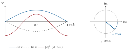
A stationary state: the spatial profile

\varphi(x)

(here the ground state of a well) multiplied by a phasor turning at the rate

E/\hbar

; real and imaginary parts rotate into each other while

|\psi|^2

stands still.

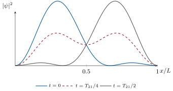
A superposition of the two lowest states of a well: the density sloshes from one side to the other at the Bohr frequency (E_2 - E_1)/h — an oscillating charge, hence () a radiating dipole at exactly the frequency of the spectral line. — A superposition of the two lowest states of a well: the density sloshes from one side to the other at the Bohr frequency $(E_2 - E_1)/h$ — an oscillating charge, hence (Chapter 17) a radiating dipole at exactly the frequency of the spectral line.

30.5 The free particle: plane waves and wave packets

Proposition 30.8 (Free particle)

For $V = 0$ the stationary states are the plane waves $\eu^{\iu(kx - \omega t)}$ with

E = \hbar\omega = \frac{\hbar^2k^2}{2m}, \qquad v_\varphi = \frac{\omega}{k} = \frac{\hbar k}{2m}, \qquad v_{\text{g}} = \frac{\dd\omega}{\dd k} = \frac{\hbar k}{m} = \frac{p}{m} :

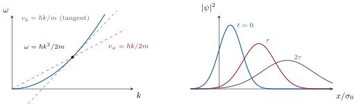
matter waves are dispersive; the phase velocity has no physical meaning, the group velocity is the particle’s velocity. A plane wave is not normalisable — a particle of perfectly sharp momentum is spread over all space — so a real particle is a wave packet, a superposition of plane waves over a band $\Delta k$ , localised over $\Delta x \sim 1/\Delta k$ , moving at $v_{\text{g}}$ and spreading: a Gaussian packet of initial width $\sigma_0$ has at time $t$ the width

\sigma(t) = \sigma_0\sqrt{1 + \Big(\frac{\hbar t}{2m\sigma_0^2}\Big)^2}, \qquad \tau = \frac{2m\sigma_0^2}{\hbar} ,

and satisfies $\Delta x\,\Delta p = \hbar/2$ at $t = 0$ (the minimum allowed) and more later.

Proof. The dispersion relation follows from the equation; $v_{\text{g}}$ as in Chapter 8. The spreading formula comes from the Fourier synthesis of the packet — each component $\eu^{\iu kx}$ picks up the phase $\eu^{-\iu\hbar k^2t/2m}$ , and the Gaussian integral with a complex coefficient gives a Gaussian of growing width; the Fourier integral is the tool of the Year 3 mathematics volume and we admit the result. Physically: the packet contains momenta spread over $\Delta p = \hbar/2\sigma_0$ , hence velocities spread over $\Delta v = \hbar/2m\sigma_0$ , and after $t$ the faster components have outrun the slower by $\Delta v\,t$ — the formula says exactly this. ∎

Left: the free particle’s dispersion curve, with the group velocity (tangent) and the phase velocity (chord to the origin), half of it. Right: a Gaussian packet moving at v_ g and spreading — its width √2 times larger after = 2m _02/, its peak lower, its area constant. — Left: the free particle’s dispersion curve, with the group velocity (tangent) and the phase velocity (chord to the origin), half of it. Right: a Gaussian packet moving at $v_{\text{g}}$ and spreading — its width $\sqrt2$ times larger after $\tau = 2m\sigma_0^2/\hbar$ , its peak lower, its area constant.

Example 30.9 (Who spreads)

An electron localised within $\sigma_0 = 1\,\mathrm{nm}$ : $\tau = 2m\sigma_0^2/\hbar = 1.7 \times 10^{-14}\,\mathrm{s}$ — after one nanosecond its packet is $60\,\text{µ}\mathrm{m}$ wide: an electron left alone does not stay put; bound in an atom it does not spread because the potential holds it (a stationary state). A dust grain of $1 \times 10^{-15}\,\mathrm{kg}$ localised to $1\,\text{µ}\mathrm{m}$ : $\tau = 2 \times 10^{7}\,\mathrm{s}$ , eight months; a bullet: longer than the age of the universe. The quantum spreading is real, and invisible for anything one can see.

Remark 30.10 (Energy and time)

A state that exists only during $\Delta t$ — an excited atom of lifetime $\tau$ , a wave train of length $c\tau$ — is a superposition of energies spread over $\Delta E \sim \hbar/\Delta t$ : the Fourier relation of Chapter 18 between the duration of a train and its spectral width, now applied to $E = \hbar\omega$ . An atomic level of lifetime $10\,\mathrm{ns}$ has a width $\Delta E = 7 \times 10^{-8}\,\mathrm{eV}$ , a natural linewidth of $16\,\mathrm{MHz}$ ; the Doppler width of Chapter 23 ( $1.5\,\mathrm{GHz}$ ) hides it in a gas, but not in a cold atom or an ion at rest.

Method 30.11 (Working with wave functions)

(1) Normalise; probabilities are $\int|\psi|^2$ over the region. (2) Time-independent $V$ : look for $\varphi(x)\eu^{-\iu Et/\hbar}$ , solve the stationary equation, impose the boundary conditions — the levels. (3) Superpose stationary states for the evolution; two levels beat at $(E_2 - E_1)/h$ . (4) Free motion: $v_{\text{g}} = p/m$ , spreading time $2m\sigma_0^2/\hbar$ . (5) Currents: $j = (\hbar/m)\operatorname{Im}(\psi^*\psi')$ ; for $A\eu^{\iu kx} + B\eu^{-\iu kx}$ , $j = (|A|^2 - |B|^2)\hbar k/m$ (no cross term). (6) Classical limit: Ehrenfest, and $\lambda$ against the size of the apparatus.

30.6 Exercises

Exercise 30.1 ★

De Broglie wavelengths: an electron at $100\,\mathrm{eV}$ , $10\,\mathrm{keV}$ , $100\,\mathrm{keV}$ (use $p = \sqrt{2mE}$ , then say why the last needs a correction); a thermal neutron ( $25\,\mathrm{meV}$ , $m = 1.67 \times 10^{-27}\,\mathrm{kg}$ ); a C $_{60}$ molecule ( $m = 1.2 \times 10^{-24}\,\mathrm{kg}$ ) at $200\,\mathrm{m}/\mathrm{s}$ ; a tennis ball. Which of these show interference?

Solution

Solution of Exercise 30.1.

$h/\sqrt{2mE}$ : $0.123\,\mathrm{nm}$ , $12.3\,\mathrm{pm}$ , $3.9\,\mathrm{pm}$ (at $100\,\mathrm{keV}$ the kinetic energy is a fifth of $mc^2$ ; the relativistic momentum gives $3.7\,\mathrm{pm}$ ); neutron $0.18\,\mathrm{nm}$ ; C $_{60}$ $2.8\,\mathrm{pm}$ ; tennis ball $\sim 10^{-34}\,\mathrm{m}$ . All but the ball have shown interference.

Exercise 30.2 ★

$\psi(x) = A\eu^{-x^2/2a^2}$ : $A$ (use $\int\eu^{-u^2}\dd u = \sqrt\pi$ ); $\langle x\rangle$ , $\Delta x$ ; probability of finding the particle in $|x| < a$ ( $\operatorname{erf}(1) = 0.84$ ) and in $|x| < 2a$ ( $0.9995$ ).

Solution

Solution of Exercise 30.2.

$A = (\pi a^2)^{-1/4}$ ; $\langle x\rangle = 0$ , $\Delta x = a/\sqrt2$ ; $0.84$ ; $0.9995$ .

Exercise 30.3 ★

Check that $\varphi(x)\eu^{-\iu Et/\hbar}$ solves the equation when $\varphi$ solves the stationary one. Frequency of the phasor for $E = 1\,\mathrm{eV}$ ; for a superposition of two levels $2\,\mathrm{eV}$ apart, frequency and wavelength of the oscillation of $|\psi|^2$ — and of the light emitted.

Solution

Solution of Exercise 30.3.

Substitution gives $E\varphi = -(\hbar^2/2m)\varphi'' + V\varphi$ . $E/h = 2.4 \times 10^{14}\,\mathrm{Hz}$ ; $4.8 \times 10^{14}\,\mathrm{Hz}$ , $620\,\mathrm{nm}$ : the red light the transition emits.

Exercise 30.4 ★

Spreading time $\tau = 2m\sigma_0^2/\hbar$ and width after $1\,\mathrm{ns}$ and $1\,\mathrm{s}$ : an electron with $\sigma_0 = 1\,\mathrm{nm}$ and $\sigma_0 = 1\,\mathrm{mm}$ ; a proton with $\sigma_0 = 1\,\mathrm{nm}$ ; a grain of $1 \times 10^{-12}\,\mathrm{kg}$ with $\sigma_0 = 1\,\text{µ}\mathrm{m}$ . Why do objects stay where they are put?

Solution

Solution of Exercise 30.4.

Electron, $1\,\mathrm{nm}$ : $\tau = 1.7 \times 10^{-14}\,\mathrm{s}$ , $60\,\text{µ}\mathrm{m}$ after $1\,\mathrm{ns}$ , $60\,\mathrm{km}$ after $1\,\mathrm{s}$ ; $1\,\mathrm{mm}$ : $\tau = 17\,\mathrm{s}$ , unchanged after $1\,\mathrm{ns}$ , $+0.2\%$ after $1\,\mathrm{s}$ ; proton, $1\,\mathrm{nm}$ : $\tau = 3.2 \times 10^{-11}\,\mathrm{s}$ , $30\,\mathrm{nm}$ , $30\,\mathrm{m}$ ; grain: $\tau = 600$ years. For visible objects $\tau$ is astronomical — and their surroundings keep localising them.

Exercise 30.5 ★★

Current. (a) Derive the continuity equation. (b) $j$ for $A\eu^{\iu kx}$ , for $A\sin kx$ , for $A\eu^{\iu kx} + B\eu^{-\iu kx}$ . (c) Why is the absence of a cross term in the last case the statement that reflected and incident fluxes simply subtract? (d) Show that for a real wave function $j = 0$ : a bound stationary state carries no current.

Solution

Solution of Exercise 30.5.

(a) Proposition 30.5. (b) $|A|^2\hbar k/m$ ; $0$ ; $(|A|^2 - |B|^2)\hbar k/m$ . (c) The incident and reflected fluxes subtract with no interference term: transmission and reflection coefficients can be defined from fluxes. (d) $\psi^*\psi'$ real, its imaginary part zero.

Exercise 30.6 ★★

A Gaussian packet. $\psi(x,0) = A\eu^{\iu k_0x}\eu^{-x^2/4\sigma^2}$ . (a) $A$ , $\langle x\rangle$ , $\Delta x$ . (b) $\langle p\rangle$ with $\hat p = -\iu\hbar\partial_x$ . (c) Admitting $\Delta p = \hbar/2\sigma$ , check $\Delta x\Delta p = \hbar/2$ . (d) Prove $\dd\langle x\rangle/\dd t = \langle p\rangle/m$ from the continuity equation.

Solution

Solution of Exercise 30.6.

(a) $A = (2\pi\sigma^2)^{-1/4}$ , $\langle x\rangle = 0$ , $\Delta x = \sigma$ . (b) $\hbar k_0$ . (c) $\sigma \times \hbar/2\sigma = \hbar/2$ . (d) $\dd\langle x\rangle/\dd t = \int x\, \partial_t\rho = -\int x\,\partial_xj = \int j = (\hbar/m)\operatorname{Im}\int\psi^* \psi' = \langle p\rangle/m$ .

Exercise 30.7 ★★

Electrons in a tube. Electrons accelerated through $100\,\mathrm{V}$ cross $30\,\mathrm{cm}$ . (a) Speed, wavelength, time of flight. (b) Phase and group velocities; which is the electron’s? (c) A packet initially $10\,\text{µ}\mathrm{m}$ wide: spreading time, width at arrival. (d) Diffraction by a $0.3\,\mathrm{mm}$ aperture on the way: angular spread and spot on the screen. Is the ray picture valid?

Solution

Solution of Exercise 30.7.

(a) $5.9 \times 10^{6}\,\mathrm{m}/\mathrm{s}$ , $0.123\,\mathrm{nm}$ , $51\,\mathrm{ns}$ . (b) $v_\varphi = 3.0 \times 10^{6}\,\mathrm{m}/\mathrm{s}$ , $v_{\text{g}} = 5.9 \times 10^{6}\,\mathrm{m}/\mathrm{s}$ : the latter. (c) $\tau = 1.7\,\text{µ}\mathrm{s} \gg 51\,\mathrm{ns}$ : unchanged. (d) $\lambda/a = 4 \times 10^{-7}\,\mathrm{rad}$ , $0.1\,\text{µ}\mathrm{m}$ : rays are fine.

Exercise 30.8 ★★

Phases. (a) Show that $\psi$ and $\eu^{\iu\theta}\psi$ give the same predictions. (b) For $\psi = (\psi_1 + \eu^{\iu\alpha}\psi_2)/\sqrt2$ , write $|\psi|^2$ and show that $\alpha$ matters. (c) In the double slit, what are $\psi_1$ and $\psi_2$ , and what fixes their relative phase at a point of the screen? (d) Why does detecting which slit the electron passed destroy the fringes (qualitative)?

Solution

Solution of Exercise 30.8.

(a) $|\psi|^2$ and every expectation value are unchanged. (b) $\tfrac12(|\psi_1|^2 + |\psi_2|^2) + \operatorname{Re}(\eu^{\iu\alpha}\psi_1^*\psi_2)$ . (c) The waves from the two slits; their relative phase is $k(r_2 - r_1)$ . (d) The detector ends in different states for the two paths; the two components no longer interfere, and the pattern is the sum of two single-slit patterns.

Exercise 30.9 ★★

Ehrenfest. (a) For $V = \tfrac12m\omega^2x^2$ , show that $\langle x\rangle$ obeys exactly $\ddot{\langle x\rangle} = -\omega^2\langle x\rangle$ . (b) For $V = mgx$ , $\langle x\rangle$ falls like a stone. (c) For a general $V$ , when is $\langle V'(x)\rangle \approx V'(\langle x\rangle)$ ? (d) A $1\,\mathrm{g}$ bead in a bowl: estimate the size of its packet needed for it to be “quantum” and compare with an atom.

Solution

Solution of Exercise 30.9.

(a) $\langle V'\rangle = m\omega^2\langle x\rangle$ : exact. (b) $\langle V'\rangle = mg$ : exact. (c) When the packet is narrow against the scale on which $V''$ varies. (d) Its wavelength at $0.1\,\mathrm{m}/\mathrm{s}$ is $10^{-29}\,\mathrm{m}$ ; the packet would have to be as wide as the bowl to matter. An atom’s thermal wavelength, $0.1\,\mathrm{nm}$ , is its own size.

Exercise 30.10 ★★★

Sloshing. In a box $0 < x < L$ with impenetrable walls the stationary states are $\varphi_n = \sqrt{2/L}\sin(n\pi x/L)$ , $E_n = n^2h^2/8mL^2$ (Chapter 31). Take $\psi = (\varphi_1\eu^{-\iu E_1t/\hbar} + \varphi_2\eu^{-\iu E_2t/\hbar})/\sqrt2$ . (a) $|\psi|^2$ as a function of time. (b) Show $\langle x\rangle = L/2 - (16L/9\pi^2)\cos\omega_{21}t$ (use $\int_0^L x\sin(\pi x/L)\sin(2\pi x/L)\dd x = -8L^2/9\pi^2$ ). (c) Electron, $L = 1\,\mathrm{nm}$ : $E_2 - E_1$ , the frequency and wavelength of the oscillation. (d) What does an oscillating charge do (Chapter 17)? Conclude on spectral lines.

Solution

Solution of Exercise 30.10.

(a) $\tfrac12(\varphi_1^2 + \varphi_2^2) + \varphi_1\varphi_2\cos\omega_{21}t$ . (b) $L/2 + \cos\omega_{21}t\int x\varphi_1\varphi_2 = L/2 - (16L/9\pi^2)\cos\omega_{21}t$ . (c) $3h^2/8mL^2 = 1.13\,\mathrm{eV}$ , $2.7 \times 10^{14}\,\mathrm{Hz}$ , $1.1\,\text{µ}\mathrm{m}$ . (d) It radiates at $\nu_{21}$ : the line; a pure stationary state has no oscillating dipole and does not radiate.

Exercise 30.11 ★★★

Spreading, derived. The packet $\psi(x,0) \propto \eu^{-x^2/4\sigma_0^2}$ is the superposition $\int g(k)\eu^{\iu kx}\dd k$ with $g(k) \propto \eu^{-\sigma_0^2k^2}$ (admitted: the Fourier transform of a Gaussian is a Gaussian, width $1/2\sigma_0$ in $k$ ). (a) Write $\psi(x,t)$ by giving each component its phase $\eu^{-\iu\hbar k^2t/2m}$ . (b) Complete the square in the exponent and admit $\int\eu^{-\alpha k^2 + \beta k}\dd k = \sqrt{\pi/\alpha}\, \eu^{\beta^2/4\alpha}$ for complex $\alpha$ with positive real part: show $|\psi|^2$ is a Gaussian of width $\sigma(t) = \sigma_0\sqrt{1 + (\hbar t/2m \sigma_0^2)^2}$ . (c) Interpret $\tau$ via $\Delta v = \Delta p/m$ . (d) Why does a packet of photons in vacuum not spread?

Solution

Solution of Exercise 30.11.

(a) $\psi \propto \int\eu^{-\sigma_0^2k^2}\eu^{\iu(kx - \hbar k^2t/2m)}\dd k$ . (b) $\alpha = \sigma_0^2 + \iu\hbar t/2m$ , $\beta = \iu x$ : $|\psi|^2 \propto \exp[-x^2/2\sigma_0^2(1 + (\hbar t/2m\sigma_0^2)^2)]$ . (c) $\Delta v = \hbar/2m\sigma_0$ , and $\Delta v\,\tau = \sigma_0$ . (d) $\omega = ck$ : no dispersion, all components at $c$ .

Exercise 30.12 ★★★

Energy–time. (a) A state decaying as $\eu^{-t/2\tau}\eu^{-\iu E_0t/\hbar}$ (probability $\eu^{-t/\tau}$ ) is a superposition of energies: admitting that its energy distribution is a Lorentzian of full width $\Gamma = \hbar/\tau$ , give $\Gamma$ for $\tau = 10\,\mathrm{ns}$ (atom), $1 \times 10^{-8}\,\mathrm{s}$ , $1 \times 10^{-23}\,\mathrm{s}$ (a hadronic resonance, in MeV). (b) Natural linewidth of the $10\,\mathrm{ns}$ level in frequency; compare with the Doppler width $1.5\,\mathrm{GHz}$ . (c) How does one see the natural width (cold atoms, trapped ions)? (d) Relate to the coherence length of the emitted wave train.

Solution

Solution of Exercise 30.12.

(a) $\Gamma = \hbar/\tau$ : $6.6 \times 10^{-8}\,\mathrm{eV}$ ; $6.6 \times 10^{-8}\,\mathrm{eV}$ ; $66\,\mathrm{MeV}$ . (b) $1/2\pi\tau = 16\,\mathrm{MHz}$ , a hundred times less than Doppler. (c) In cold atoms and trapped ions the Doppler width vanishes and the natural width is reached — the basis of frequency standards. (d) $c\tau = 3\,\mathrm{m}$ , the train’s length.

30.7 Problem: The electron in a tube and the spreading of a wave packet

Problem 30.1

Weekend problem — when is an electron a particle, when a wave

Data: $h = 6.63 \times 10^{-34}\,\mathrm{J}\,\mathrm{s}$ , $\hbar = 1.05 \times 10^{-34}\,\mathrm{J}\,\mathrm{s}$ , $m_{\text{e}} = 9.11 \times 10^{-31}\,\mathrm{kg}$ , $e = 1.60 \times 10^{-19}\,\mathrm{C}$ , $m_{\text{p}} = 1.67 \times 10^{-27}\,\mathrm{kg}$ .

Part I — The cathode-ray tube. Electrons leave a hot cathode with negligible energy, are accelerated through $U = 20\,\mathrm{kV}$ , pass a $0.3\,\mathrm{mm}$ aperture, and hit a screen $40\,\mathrm{cm}$ away.

Speed and momentum (non-relativistic); de Broglie wavelength.
The kinetic energy is $4\%$ of $mc^2$ : is the non-relativistic treatment acceptable for this problem?
Time of flight to the screen.
Diffraction by the aperture: angular spread $\sim\lambda/a$ and the spot it produces on the screen; compare with a pixel ( $0.3\,\mathrm{mm}$ ).
Heisenberg at the aperture: $\Delta p_y \gtrsim \hbar/2a$ gives the same spread — check.
A packet $0.3\,\mathrm{mm}$ wide along the beam: spreading time $2m\sigma_0^2/\hbar$ and width at the screen.
Deflection plates apply a transverse force: by Ehrenfest, how does $\langle y\rangle$ move? Conclude that the tube is a classical device.
Phase velocity of the electron wave; why is it no paradox that it differs from the electron’s speed?

Part II — Wave packets.

For a Gaussian packet of width $\sigma_0$ : $\Delta p$ and the velocity spread $\Delta v$ .
Spreading time for an electron with $\sigma_0 = 0.1\,\mathrm{nm}$ , $1\,\mathrm{nm}$ , $1\,\text{µ}\mathrm{m}$ ; for a proton with $1\,\mathrm{nm}$ ; for a virus ( $1 \times 10^{-17}\,\mathrm{kg}$ ) with $10\,\mathrm{nm}$ .
An electron in a hydrogen atom is localised to $0.1\,\mathrm{nm}$ and does not spread: why?
A free electron at $1\,\mathrm{eV}$ with $\sigma_0 = 1\,\mathrm{nm}$ : how far does it travel before its width doubles? Compare with the wavelength.
In a metal, conduction electrons are waves of $\lambda \approx 0.5\,\mathrm{nm}$ over the whole crystal: in what sense are they “delocalised”?
An electron microscope at $100\,\mathrm{keV}$ has $\lambda \approx 4\,\mathrm{pm}$ , yet resolves only $0.1\,\mathrm{nm}$ : why (its magnetic lenses accept a half-angle of about $10\,\mathrm{mrad}$ )?
Give the criterion that decides whether an object must be treated with a wave function or with Newton.

Part III — Stationary states and transitions. An electron is confined in $0 < x < L = 1\,\mathrm{nm}$ ; $\varphi_n = \sqrt{2/L}\sin(n\pi x/L)$ , $E_n = n^2h^2/8mL^2$ .

$E_1$ , $E_2$ , $E_3$ in electronvolts; the Bohr frequencies $\nu_{21}$ , $\nu_{31}$ and the wavelengths.
Check that $|\varphi_n\eu^{-\iu E_nt/\hbar}|^2$ is time-independent; where is the electron most likely in the ground state?
For $\psi = (\varphi_1\eu^{-\iu E_1t/\hbar} + \varphi_2\eu^{-\iu E_2t/\hbar})/ \sqrt2$ : $|\psi|^2$ at $t = 0$ and $t = T_{21}/2$ ; sketch.
$\langle x\rangle(t)$ (given $\int_0^Lx\varphi_1\varphi_2\dd x = -16L/9\pi^2$ ): amplitude of the sloshing.
The oscillating dipole $e\langle x\rangle$ radiates: at which frequency, and what does that say about spectral lines and about the stability of stationary states?
Energy of the state $\psi$ : is it $E_1$ , $E_2$ , or something else? What does a measurement give?

Part IV — Interpretation.

In the single-electron double-slit experiment, what is random and what is not?
Write the probability current of $A\eu^{\iu kx}$ and relate it to a beam of $n$ electrons per unit length at speed $v$ .
Why must the Schrödinger equation be complex and first order in time (two reasons)?
Summarise in five lines: the wave function, the equation, the stationary states, the packet, the classical limit.

Solution

Solution of Problem 30.1.

1. $v = \sqrt{2eU/m} = 8.4 \times 10^{7}\,\mathrm{m}/\mathrm{s}$ ; $p = 7.6 \times 10^{-23}\,\mathrm{kg}\,\mathrm{m}/\mathrm{s}$ ; $\lambda = 8.7\,\mathrm{pm}$ .

2. Errors of a few per cent: acceptable for estimates ( $\lambda = 8.6\,\mathrm{pm}$ exactly).

3. $4.8\,\mathrm{ns}$ .

4. $\lambda/a = 3 \times 10^{-8}\,\mathrm{rad}$ : $12\,\mathrm{nm}$ — $10^4$ times smaller than a pixel.

5. $\Delta\theta = \Delta p_y/p \sim \hbar/2ap = \lambda/4\pi a$ : the same order.

6. $\tau = 1.6\,\mathrm{ms} \gg 4.8\,\mathrm{ns}$ : unchanged.

7. $\dd\langle p_y\rangle/\dd t = eE$ exactly for a uniform field: $\langle y\rangle$ follows the classical parabola; the tube is a classical instrument.

8. $v/2 = 4.2 \times 10^{7}\,\mathrm{m}/\mathrm{s}$ ; only the group velocity is observable; a plane wave’s phase carries no signal (and depends on the arbitrary zero of energy).

9. $\Delta p = \hbar/2\sigma_0$ , $\Delta v = \hbar/2m\sigma_0$ .

10. $1.7 \times 10^{-16}\,\mathrm{s}$ , $1.7 \times 10^{-14}\,\mathrm{s}$ , $1.7 \times 10^{-8}\,\mathrm{s}$ ; proton $3.2 \times 10^{-11}\,\mathrm{s}$ ; virus $20\,\mathrm{s}$ .

11. It is in a stationary state: the potential holds the packet; $|\varphi|^2$ does not move.

12. $v = 5.9 \times 10^{5}\,\mathrm{m}/\mathrm{s}$ ; doubling at $t = \sqrt3\tau = 2.9 \times 10^{-14}\,\mathrm{s}$ : $17\,\mathrm{nm}$ , some fourteen wavelengths.

13. Their wave functions extend over the whole crystal: a definite momentum, no definite position.

14. Resolution $\sim\lambda/\alpha = 4\,\mathrm{pm}/0.01 = 0.4\,\mathrm{nm}$ : the aberrations of magnetic lenses limit the aperture, not the wavelength.

15. Compare $\lambda$ with the sizes in play (apertures, the scale of $V$ ), and the spreading time with the observation time.

16. $0.38\,$ , $1.50\,$ , $3.38\,\mathrm{eV}$ ; $\nu_{21} = 2.7 \times 10^{14}\,\mathrm{Hz}$ ( $1.1\,\text{µ}\mathrm{m}$ ), $\nu_{31} = 7.3 \times 10^{14}\,\mathrm{Hz}$ ( $410\,\mathrm{nm}$ ).

17. The phasor has modulus one; at $x = L/2$ .

18. At $t = 0$ the density piles up on the left half, at $T_{21}/2$ on the right.

19. $\langle x\rangle = L/2 - (16L/9\pi^2)\cos\omega_{21}t$ : amplitude $0.18L = 0.18\,\mathrm{nm}$ .

20. At $\nu_{21}$ : the spectral line; a stationary state has no oscillating dipole and is stable; the superposition radiates its way down to $\varphi_1$ .

21. Not definite: $\langle E\rangle = (E_1 + E_2)/2 = 0.94\,\mathrm{eV}$ ; a measurement gives $E_1$ or $E_2$ , each with probability one half.

22. Random: where each electron lands; not random: the pattern $|\psi|^2$ that the landings build.

23. $j = |A|^2\hbar k/m$ : with $|A|^2 = n$ electrons per unit length, $nv$ electrons per second.

24. First order so that $\psi(x,0)$ is a complete description that fixes the future; complex so that a definite energy has the single time dependence $\eu^{-\iu Et/\hbar}$ and $E = p^2/2m$ comes out.

25. $\psi$ is the amplitude whose square is the probability; it obeys Schrödinger’s linear equation; stationary states carry a phasor and fixed densities; a free packet moves at $p/m$ and spreads in $2m\sigma_0^2/\hbar$ ; Ehrenfest gives Newton back for the large.

Terms defined in this chapter

Wave function and Born’s rule

See all 393 terms in the glossary