University Physics — Year 2 · Bachelor Year 2

11Maxwell’s Equations

In 1865 James Clerk Maxwell wrote down the laws that Coulomb, Ampère and Faraday had found one by one, added to Ampère’s a term that no experiment had yet demanded, and found that his equations admitted waves travelling at a speed he could compute from the constants of electricity and magnetism — the speed of light. Electricity, magnetism and optics were one subject. The Year 1 volume stated the laws as integrals over surfaces and loops; this chapter writes them as four local equations valid at every point and every instant, with the vector operators that make such a writing possible, and draws the first consequences: the displacement current, the potentials, the behaviour of the fields at an interface, and the approximations under which the circuits of the Year 1 volume are exact.

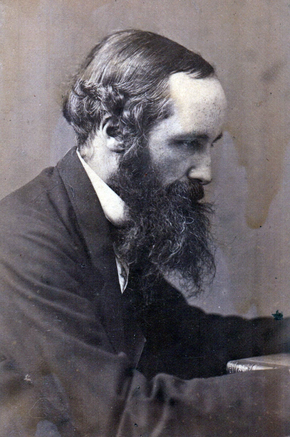
James Clerk Maxwell (1831–1879), who wrote the four equations of this chapter and read in them the existence of electromagnetic waves travelling at the speed of light.

11.1 Vector operators

Definition 11.1 (Gradient, divergence, curl, Laplacian)

For a scalar field $f$ and a vector field $\vect A$ , in Cartesian coordinates with the symbolic vector $\vect\nabla = (\partial_x, \partial_y, \partial_z)$ :

\begin{align*} \operatorname{\vect{grad}}f &= \vect\nabla f = (\partial_xf,\ \partial_yf,\ \partial_zf) ,\\ \operatorname{div}\vect A &= \vect\nabla\cdot\vect A = \partial_xA_x + \partial_yA_y + \partial_zA_z ,\\ \operatorname{\vect{curl}}\vect A &= \vect\nabla\wedge\vect A = (\partial_yA_z - \partial_zA_y,\ \partial_zA_x - \partial_xA_z,\ \partial_xA_y - \partial_yA_x) ,\\ \Delta f &= \operatorname{div}\operatorname{\vect{grad}}f = \partial_x^2f + \partial_y^2f + \partial_z^2f , \end{align*}

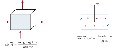
and $\Delta\vect A$ is the Laplacian taken on each Cartesian component. Their meaning is independent of coordinates: $\operatorname{\vect{grad}}f \cdot\dd\vect l = \dd f$ is the change of $f$ along $\dd\vect l$ ; $\operatorname{div} \vect A$ is the outgoing flux of $\vect A$ through the surface of a small volume, per unit volume; $\operatorname{\vect{curl}}\vect A\cdot\vect n$ is the circulation of $\vect A$ around a small loop of normal $\vect n$ , per unit area.

Theorem 11.2 (Divergence and Stokes theorems)

For a closed surface $\Sigma$ bounding the volume $V$ , and an oriented closed curve $C$ bounding the surface $S$ (normal $\vect n$ given by the right-hand rule),

\iint_\Sigma\vect A\cdot\vect n\,\dd S = \iiint_V\operatorname{div}\vect A\,\dd\tau , \qquad \oint_C\vect A\cdot\dd\vect l = \iint_S\operatorname{\vect{curl}}\vect A\cdot\vect n\,\dd S .

Proof. Admitted at this level. ∎

Remark 11.3 (What is admitted and why it is believable)

Both theorems are proved in the Year 3 mathematics volume; the mathematics volume of this year stops at their plane version (Green–Riemann) and at multiple integrals. Their content, however, is the one we used in Chapter 2: tile the volume with small boxes (the loop’s surface with small loops) — the fluxes through the interior faces (the circulations along the interior edges) cancel in pairs, and only the boundary remains. Two identities follow from the definitions and are used constantly: $\operatorname{\vect{curl}}\operatorname{\vect{grad}}f = \vect 0$ , $\operatorname{div}\operatorname{\vect{curl}}\vect A = 0$ , and $\operatorname{\vect{curl}}\operatorname{\vect{curl}}\vect A = \operatorname{\vect{grad}} \operatorname{div}\vect A - \Delta\vect A$ . For fields with a symmetry, the useful formulas are: for a radial field $A_r(r)\vect e_r$ , $\operatorname{div} = \frac1{r^2}\partial_r(r^2A_r)$ (spherical) or $\frac1r\partial_r(rA_r)$ (cylindrical); for an azimuthal field $A_\theta(r)\vect e_\theta$ around an axis, $(\operatorname{\vect{curl}})_z = \frac1r\partial_r(rA_\theta)$ ; and for $f(r)$ , $\Delta f = \frac1{r^2}\partial_r(r^2\partial_rf) = \frac1r\partial_r^2(rf)$ (spherical), $\frac1r\partial_r(r\partial_rf)$ (cylindrical).

The two operators of the Maxwell equations, read geometrically: the divergence measures how much a field flows out of a small volume, the curl how much it circulates around a small loop.

11.2 The four equations

Theorem 11.4 (Maxwell’s equations)

In vacuum (and in matter described by its total charge and current densities $\rho$ and $\vect j$ ), the electric and magnetic fields obey, at every point and every time,

\begin{align*} \operatorname{div}\vect E &= \frac\rho{\varepsilon_0} &&\text{(Maxwell--Gauss)} , & \operatorname{\vect{curl}}\vect E &= -\frac{\partial\vect B}{\partial t} &&\text{(Maxwell--Faraday)} ,\\ \operatorname{div}\vect B &= 0 &&\text{(Maxwell--flux)} , & \operatorname{\vect{curl}}\vect B &= \mu_0\vect j + \mu_0\varepsilon_0\frac{\partial\vect E}{\partial t} &&\text{(Maxwell--Ampère)} , \end{align*}

with $\varepsilon_0 = 8.85 \times 10^{-12}\,\mathrm{F}/\mathrm{m}$ , $\mu_0 = 4\pi \times 1 \times 10^{-7}\,\mathrm{H}/\mathrm{m}$ (and $\varepsilon_0\mu_0 = 1/c^2$ ). The fields act on charges through the Lorentz force $\vect F = q(\vect E + \vect v\wedge\vect B)$ . The term $\varepsilon_0\partial_t\vect E$ is Maxwell’s displacement current density.

Equivalence with the integral laws of the Year 1 volume. Apply the divergence theorem to the first two: $\iint_\Sigma\vect E\cdot \vect n\,\dd S = Q_{\text{int}}/\varepsilon_0$ (Gauss) and the flux of $\vect B$ through any closed surface is zero. Apply Stokes to the last two: $\oint_C\vect E\cdot\dd\vect l = -\dd\Phi_B/\dd t$ (Faraday, for a fixed loop) and $\oint_C\vect B\cdot\dd\vect l = \mu_0I_{\text{enc}} + \mu_0\varepsilon_0\,\dd\Phi_E/\dd t$ (Ampère, completed). Conversely the integral laws, holding for every volume and loop, imply the local ones. The local equations are thus the Year 1 laws plus one new term, justified below; they are taken as the postulates of electromagnetism. ∎

Proposition 11.5 (Why the displacement current is necessary)

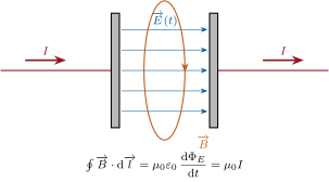
Taking the divergence of the Maxwell–Ampère equation and using $\operatorname{div}\operatorname{\vect{curl}} = 0$ and Maxwell–Gauss gives

0 = \mu_0\operatorname{div}\vect j + \mu_0\varepsilon_0\,\partial_t\operatorname{div}\vect E = \mu_0\Bigl(\operatorname{div}\vect j + \frac{\partial\rho}{\partial t}\Bigr) :

the equations contain the conservation of charge. Without the displacement term they would require $\operatorname{div}\vect j = 0$ always — false in a charging capacitor, where the conduction current stops at the plate. There, between the plates, $\varepsilon_0\partial_t\vect E$ carries exactly the current that arrives in the wire, and the magnetic field circulates around the gap as around a wire.

Proof. Divergence of both sides, as stated; for the capacitor, the flux of $\varepsilon_0\partial_t\vect E$ through a surface between the plates is $\varepsilon_0S\,\dd E/\dd t = \dd Q/\dd t = I$ . ∎

Example 11.6 (The field inside a charging capacitor)

Circular plates of radius $R$ , separation $d \ll R$ , charged by a current $I$ : between them $E = Q/\varepsilon_0\pi R^2$ is uniform and grows at $\dd E/ \dd t = I/\varepsilon_0\pi R^2$ . By symmetry $\vect B = B(r)\vect e_\theta$ ; Ampère–Maxwell on a circle of radius $r < R$ (no conduction current crosses it): $2\pi rB = \mu_0\varepsilon_0\pi r^2\,\dd E/\dd t$ , so $B = \mu_0Ir/2\pi R^2$ — the field of a uniform current $I$ spread over the disk, continuous at $r = R$ with the wire’s $\mu_0I/2\pi r$ outside. For $I = 1\,\mathrm{A}$ , $R = 5\,\mathrm{cm}$ : $B(R) = 4\,\text{µ}\mathrm{T}$ , measurable; Maxwell’s term is real.

A capacitor being charged: no charge crosses the gap, but the electric flux through a loop around it grows; Maxwell’s term gives the loop the same circulation of B as if the wire continued — the displacement current. — A capacitor being charged: no charge crosses the gap, but the electric flux through a loop around it grows; Maxwell’s term gives the loop the same circulation of $\vect B$ as if the wire continued — the displacement current.

Remark 11.7 (Linearity; what the equations say)

The equations are linear in the fields and their sources: fields superpose. Two of them (Gauss, Faraday–flux) carry no sources and express structure — electric field lines start and end on charges, magnetic field lines never end; the other two say how charges and currents, and each field’s variation, create the fields. Read together, a varying $\vect B$ makes a circulating $\vect E$ and a varying $\vect E$ makes a circulating $\vect B$ : the two can sustain each other with no charge anywhere — that is the wave of Chapter 13, and the displacement current is what makes it possible.

11.3 Potentials

Proposition 11.8 (Scalar and vector potentials)

Because $\operatorname{div}\vect B = 0$ and $\operatorname{\vect{curl}}\vect E = -\partial_t \vect B$ , the fields derive from a vector potential $\vect A$ and a scalar potential $V$ :

\vect B = \operatorname{\vect{curl}}\vect A , \qquad \vect E = -\operatorname{\vect{grad}}V - \frac{\partial\vect A}{\partial t} ,

determined up to a gauge transformation $\vect A \to \vect A + \operatorname{\vect{grad}}\chi$ , $V \to V - \partial_t\chi$ , which leaves the fields unchanged. In the Coulomb gauge $\operatorname{div}\vect A = 0$ , Gauss’s law becomes Poisson’s equation

\Delta V = -\frac\rho{\varepsilon_0} ,

and in a stationary regime Ampère’s law becomes $\Delta\vect A = -\mu_0\vect j$ . In statics $V$ is the electrostatic potential of the Year 1 volume.

Proof. A divergence-free field is a curl (admitted, like the converse statement that a curl-free field is a gradient, both from the Year 2 mathematics volume for simply connected regions); then $\operatorname{\vect{curl}} (\vect E + \partial_t\vect A) = \vect 0$ , so $\vect E + \partial_t\vect A$ is a gradient. Gauge: $\operatorname{\vect{curl}}\operatorname{\vect{grad}}\chi = \vect 0$ and the $\partial_t\operatorname{\vect{grad}}\chi$ terms cancel in $\vect E$ . Poisson: $\operatorname{div} \vect E = -\Delta V - \partial_t\operatorname{div}\vect A$ . Statics: $\operatorname{\vect{curl}} \operatorname{\vect{curl}}\vect A = \operatorname{\vect{grad}}\operatorname{div}\vect A - \Delta\vect A = \mu_0\vect j$ . ∎

Example 11.9 (Two vector potentials)

A uniform field $\vect B_0$ derives from $\vect A = \tfrac12\vect B_0\wedge\vect r$ (check: $\operatorname{\vect{curl}}(\tfrac12\vect B_0\wedge\vect r) = \vect B_0$ , and $\operatorname{div}\vect A = 0$ ); inside an infinite solenoid this is $A_\theta = Br/2$ , outside $A_\theta = BR^2/2r$ — a potential that does not vanish where the field does, and whose circulation along a loop is the flux of $\vect B$ through it: $\oint\vect A\cdot\dd\vect l = \Phi_B$ (Stokes). Faraday’s law then reads $\vect E = -\partial_t\vect A$ for the induced field.

11.4 The fields at an interface

Proposition 11.10 (Boundary relations)

Across a surface carrying the surface charge density $\sigma$ and the surface current density $\vect j_s$ ( $\mathrm{A}/\mathrm{m}$ ), with $\vect n_{12}$ the unit normal from medium 1 to medium 2,

\vect E_2 - \vect E_1 = \frac\sigma{\varepsilon_0}\,\vect n_{12} , \qquad \vect B_2 - \vect B_1 = \mu_0\,\vect j_s\wedge\vect n_{12} :

the tangential component of $\vect E$ and the normal component of $\vect B$ are continuous; the normal component of $\vect E$ jumps by $\sigma/\varepsilon_0$ , the tangential component of $\vect B$ by $\mu_0j_s$ . At the surface of a perfect conductor ( $\vect E = \vect B = \vect 0$ inside, in the cases of Chapter 15), $\vect E$ is normal and equal to $\sigma\vect n/ \varepsilon_0$ , $\vect B$ is tangential and equal to $\mu_0\vect j_s\wedge\vect n$ .

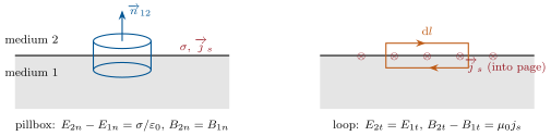
Proof. Normal components: Gauss’s and the flux law on a flat pillbox straddling the surface, of area $\dd S$ and vanishing height: $(E_{2n} - E_{1n})\dd S = \sigma\dd S/\varepsilon_0$ , $(B_{2n} - B_{1n})\dd S = 0$ . Tangential components: Faraday’s and Ampère’s laws on a small rectangle straddling the surface, of length $\dd l$ and vanishing height: the fluxes of $\partial_t\vect B$ and $\partial_t\vect E$ through the rectangle vanish with its area, but a surface current $j_s\,\dd l$ crosses it: $(E_{2t} - E_{1t})\dd l = 0$ , $(B_{2t} - B_{1t})\dd l = \mu_0j_s\dd l$ for the tangential direction perpendicular to $\vect j_s$ . ∎

The boundary relations come from the integral laws applied to a flat pillbox and a thin loop straddling the interface: surface charge makes the normal E jump, surface current makes the tangential B jump; the other components are continuous. — The boundary relations come from the integral laws applied to a flat pillbox and a thin loop straddling the interface: surface charge makes the normal $\vect E$ jump, surface current makes the tangential $\vect B$ jump; the other components are continuous.

Example 11.11 (Charged plane, current sheet, solenoid)

A plane with $\sigma$ alone in space: by symmetry $\vect E = \pm E\vect n$ on its two sides, and the jump $2E = \sigma/\varepsilon_0$ gives $E = \sigma/2\varepsilon_0$ — the Year 1 result in one line. A plane sheet of current $j_s$ : $B = \mu_0j_s/2$ on each side, antiparallel. A long solenoid of $n$ turns per metre carrying $I$ is a cylindrical current sheet $j_s = nI$ : the jump $\mu_0nI$ across it, with $B = 0$ outside, gives $B = \mu_0nI$ inside.

11.5 Quasi-stationary regimes

Definition 11.12 (The quasi-stationary approximations)

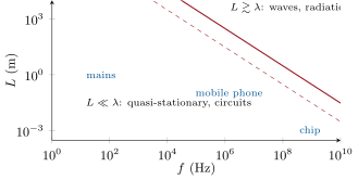
A system of size $L$ driven at frequency $f$ is quasi-stationary when $L \ll \lambda = c/f$ : the time $L/c$ the fields need to cross it is negligible compared with the period, and all its points "see" the sources at the same instant. Two limits are used:

the magnetic quasi-stationary regime (circuits with currents, coils, transformers, induction): the displacement current is dropped from Ampère’s law, $\operatorname{\vect{curl}}\vect B = \mu_0\vect j$ (so $\operatorname{div}\vect j = 0$ and currents flow in closed circuits), while Faraday’s law is kept in full;
the electric quasi-stationary regime (a charging capacitor): Faraday’s term is dropped, $\vect E$ is the electrostatic field of the instantaneous charges, while the displacement current is kept to find $\vect B$ .

Justification. In the magnetic regime, compare the two terms of Ampère’s law in a conductor: $\mu_0\varepsilon_0\partial_t E \sim \mu_0\varepsilon_0\omega E$ against $\mu_0\gamma E$ , a ratio $\varepsilon_0\omega/\gamma = \omega\tau_r \sim 10^{-17}$ at $50\,\mathrm{Hz}$ in copper; outside the conductor the displacement current is of order $\varepsilon_0\omega E$ with $E \sim \omega AB$ , i.e. smaller than the conduction current’s effect by $(\omega L/c)^2 = (L/\lambda)^2 \times 4\pi^2$ . In the electric regime the induced field $\omega BL \sim \omega^2\varepsilon_0\mu_0L^2E$ is smaller than $E$ by the same $(L/\lambda)^2$ . ∎

Example 11.13 (Circuits and antennas)

A mains circuit at $50\,\mathrm{Hz}$ ( $\lambda = 6000\,\mathrm{km}$ ) is quasi-stationary up to the size of a country — it is why Kirchhoff’s laws and the transformer work. A $10\,\mathrm{cm}$ circuit is quasi-stationary up to some $100\,\mathrm{MHz}$ ; at $1\,\mathrm{GHz}$ ( $\lambda = 30\,\mathrm{cm}$ ) its wires are antennas, currents differ along a wire, and the circuit radiates: the domain of Chapter 17 and of microwave design, where a track on a board is a transmission line.

Size against frequency: below the line L = /10 (dashed) a device is quasi-stationary and the circuit laws hold; near and above L = the fields propagate, and the device radiates. — Size against frequency: below the line $L = \lambda/10$ (dashed) a device is quasi-stationary and the circuit laws hold; near and above $L = \lambda$ the fields propagate, and the device radiates.

Method 11.14 (Using the local equations)

(1) Use the symmetries and invariances of the sources to fix the direction and the variables of the fields (as in the Year 1 volume). (2) Choose the form: integral (Gauss, Ampère on a well-chosen surface or loop) when there is enough symmetry; local when you need a differential equation (Poisson for $V$ , the diffusion or wave equation for the fields). (3) In a time-dependent problem decide the regime: static, quasi-stationary magnetic or electric, or full Maxwell. (4) At interfaces, use the boundary relations — they are the only place where surface charges and currents enter. (5) Check $\operatorname{div}\vect B = 0$ and the dimensions.

11.6 Exercises

Exercise 11.1 ★

Compute the divergence and the curl of (a) $\vect A = (x, y, z)$ ; (b) $\vect A = (-y, x, 0)$ ; (c) $\vect A = (yz, zx, xy)$ ; (d) $\vect A = \vect r/r^3$ (use the radial formula, $r \ne 0$ ); (e) $\vect A = (0, 0, x^2)$ . Which are gradients, which are curls, which are neither?

Solution

Solution of Exercise 11.1.

(a) $\operatorname{div} = 3$ , $\operatorname{\vect{curl}} = \vect 0$ : the gradient of $r^2/2$ . (b) $0$ and $(0, 0, 2)$ : a curl (of $-\tfrac12(x^2 + y^2)\vect e_z$ ), not a gradient. (c) $0$ and $\vect 0$ : the gradient of $xyz$ (and a curl too). (d) $\frac1{r^2}\partial_r(r^2/r^2) = 0$ , curl $\vect 0$ : the gradient of $-1/r$ . (e) $0$ and $(0, -2x, 0)$ : a curl, not a gradient.

Exercise 11.2 ★

(a) Check the dimensions of each term of the four Maxwell equations. (b) Compute $1/\sqrt{\varepsilon_0\mu_0}$ . (c) Ratio of the displacement current density to the conduction current density in copper at $50\,\mathrm{Hz}$ , in sea water ( $\gamma = 5\,\mathrm{S}/\mathrm{m}$ ) at $1\,\mathrm{GHz}$ , in glass ( $\gamma = 1 \times 10^{-12}\,\mathrm{S}/\mathrm{m}$ , $\varepsilon_0$ taken for simplicity) at $50\,\mathrm{Hz}$ : which is "a conductor" for each?

Solution

Solution of Exercise 11.2.

(a) Gauss and Faraday: both sides in $\mathrm{V}/\mathrm{m}^{2}$ (a charge density over $\varepsilon_0$ , a field gradient, a field over a time); Ampère: both sides in $\mathrm{T}/\mathrm{m}$ . (b) $1/\sqrt{8.85 \times 10^{-12} \times 1.257 \times 10^{-6}} = 3.00 \times 10^{8}\,\mathrm{m}/\mathrm{s}$ . (c) Ratio $\varepsilon_0\omega/\gamma$ : copper $5 \times 10^{-20}$ ; sea water at $1\,\mathrm{GHz}$ $1 \times 10^{-2}$ (still a conductor, just); glass at $50\,\mathrm{Hz}$ $3 \times 10^3$ : a dielectric, the displacement current dominates.

Exercise 11.3 ★

A capacitor with circular plates ( $R = 10\,\mathrm{cm}$ , $d = 2\,\mathrm{mm}$ ) is charged by $I = 0.5\,\mathrm{A}$ . Rate of change of $E$ ; displacement current density; $B$ at $r = 5\,\mathrm{cm}$ and at $r = 20\,\mathrm{cm}$ (in the plane midway between the plates); compare the latter with the field of the feeding wire at the same distance.

Solution

Solution of Exercise 11.3.

$\dd E/\dd t = I/\varepsilon_0\pi R^2 = 1.8 \times 10^{12}\,\mathrm{V}\,\mathrm{m}^{-1}\,\mathrm{s}^{-1}$ ; $j_d = I/\pi R^2 = 16\,\mathrm{A}/\mathrm{m}^{2}$ ; $B(5\,\mathrm{cm}) = \mu_0Ir/2\pi R^2 = 0.5\,\text{µ}\mathrm{T}$ ; $B(20\,\mathrm{cm}) = \mu_0I/2\pi r = 0.5\,\text{µ}\mathrm{T}$ — exactly the wire’s field.

Exercise 11.4 ★

(a) $\vect E = kx\,\vect e_x$ fills a region: charge density there. (b) Inside a ball of radius $R$ , $\vect E = (\rho_0r/3\varepsilon_0)\vect e_r$ : check with the radial divergence that $\rho = \rho_0$ , and recover the field outside from Gauss’s integral law. (c) $\vect B = B_0(y/a)\vect e_x$ : is it a possible magnetic field? What current density sustains it?

Solution

Solution of Exercise 11.4.

(a) $\rho = \varepsilon_0k$ . (b) $\frac1{r^2}\partial_r(\rho_0r^3/3\varepsilon_0) = \rho_0/\varepsilon_0$ ; outside, Gauss: $E = \rho_0R^3/3\varepsilon_0r^2$ . (c) $\operatorname{div}\vect B = 0$ : yes; $\operatorname{\vect{curl}}\vect B = -(B_0/a)\vect e_z$ : $\vect j = -(B_0/\mu_0a)\vect e_z$ , a uniform current sheet of thickness along $y$ .

Exercise 11.5 ★★

Vector potentials. (a) Show that $\vect A = \tfrac12\vect B_0\wedge\vect r$ gives $\operatorname{\vect{curl}}\vect A = \vect B_0$ and $\operatorname{div}\vect A = 0$ . (b) So does $\vect A' = B_0x\,\vect e_y$ : find the gauge function $\chi$ with $\vect A' = \vect A + \operatorname{\vect{grad}}\chi$ . (c) Solenoid of radius $R$ , field $B$ inside: check $A_\theta = Br/2$ ( $r < R$ ) and $BR^2/2r$ ( $r > R$ ) with $(\operatorname{\vect{curl}}\vect A)_z = \frac1r\partial_r(rA_\theta)$ ; continuity at $R$ . (d) Circulation of $\vect A$ on a circle of radius $r > R$ and the flux of $\vect B$ : what does this say about the induced emf in a loop outside a solenoid whose current varies?

Solution

Solution of Exercise 11.5.

(a) $\vect A = \tfrac12(B_yz - B_zy, B_zx - B_xz, B_xy - B_yx)$ : $(\operatorname{\vect{curl}} \vect A)_x = \tfrac12(B_x + B_x) = B_x$ , etc.; $\operatorname{div}\vect A = 0$ . (b) $\vect A' - \vect A = \tfrac12B_0(y, x, 0) = \operatorname{\vect{grad}}(\tfrac12B_0xy)$ . (c) $\frac1r\partial_r(Br^2/2) = B$ ; $\frac1r\partial_r(BR^2/2) = 0$ ; both equal $BR/2$ at $R$ . (d) $2\pi r\cdot BR^2/2r = \pi R^2B = \Phi$ : a loop outside the solenoid, where $\vect B = \vect 0$ , still feels $e = -\dd\Phi/\dd t$ — through $\vect E = -\partial_t\vect A$ , which does not vanish there.

Exercise 11.6 ★★

Boundary relations. (a) A conductor in electrostatic equilibrium carries $\sigma$ on its surface: field just outside (from the jump, with $\vect E = \vect 0$ inside); for $\sigma = 1\,\text{µ}\mathrm{C}/\mathrm{m}^{2}$ . (b) Two parallel planes with $+\sigma$ and $-\sigma$ : field everywhere, by the jumps. (c) A long solenoid ( $n = 2000\,\mathrm{m}^{-1}$ , $I = 5\,\mathrm{A}$ ) as a current sheet: $j_s$ , the jump of $B$ , $B$ inside. (d) A toroidal coil: why is $B$ zero outside and $\mu_0NI/2\pi r$ inside, from the same jump?

Solution

Solution of Exercise 11.6.

(a) $E = \sigma/\varepsilon_0 = 1.1 \times 10^{5}\,\mathrm{V}/\mathrm{m}$ , normal. (b) $\sigma/\varepsilon_0$ between, zero outside (each jump adds $\pm\sigma/\varepsilon_0$ ). (c) $j_s = nI = 1 \times 10^{4}\,\mathrm{A}/\mathrm{m}$ , jump $\mu_0j_s = 12.6\,\mathrm{mT} = B$ inside. (d) A loop outside the torus encloses no net current, so $B = 0$ there; inside, Ampère gives $\mu_0NI/2\pi r$ , and the jump across the winding, $\mu_0j_s = \mu_0NI/2\pi r$ , agrees.

Exercise 11.7 ★★

Poisson in one dimension. Between two plane electrodes at $x = 0$ ( $V = 0$ ) and $x = d$ ( $V = U$ ), a uniform charge density $\rho_0$ fills the gap (a space charge). (a) Solve Poisson’s equation for $V(x)$ . (b) Field $E(x)$ ; where is it zero if $\rho_0 > 0$ and large? (c) Surface charges on the two electrodes, from the boundary relation. (d) With $\rho_0 = 0$ recover the capacitor; with $U = 0$ , sketch $V$ .

Solution

Solution of Exercise 11.7.

(a) $V'' = -\rho_0/\varepsilon_0$ : $V = -\rho_0x^2/2\varepsilon_0 + (U/d + \rho_0d/2\varepsilon_0)x$ . (b) $E = \rho_0x/\varepsilon_0 - U/d - \rho_0d/2\varepsilon_0$ , zero at $x_0 = d/2 + \varepsilon_0U/\rho_0d$ — near the middle for a large space charge. (c) $\sigma(0) = \varepsilon_0E(0^+) = -\varepsilon_0U/d - \rho_0d/2$ , $\sigma(d) = -\varepsilon_0E(d^-) = \varepsilon_0U/d - \rho_0d/2$ : together $-\rho_0d$ , neutralizing the space charge. (d) $\rho_0 = 0$ : linear $V$ , uniform $E$ ; $U = 0$ : a parabola peaking at $d/2$ .

Exercise 11.8 ★★

Quasi-stationary or not. (a) $\lambda$ at $50\,\mathrm{Hz}$ , $1\,\mathrm{MHz}$ , $100\,\mathrm{MHz}$ , $2.4\,\mathrm{GHz}$ . (b) Up to what frequency is a $10\,\mathrm{cm}$ circuit quasi-stationary (criterion $L < \lambda/10$ )? A $1\,\mathrm{cm}$ chip? A $1000\,\mathrm{km}$ power grid? (c) In a capacitor of radius $R = 5\,\mathrm{cm}$ at $1\,\mathrm{MHz}$ , estimate the ratio of the induced electric field (from the varying $\vect B$ of the previous exercises) to the main field: $(\omega R/c)^2 /4$ . (d) Why is the mains frequency of a continent-wide grid a quasi-stationary problem although the grid is $1000\,\mathrm{km}$ across?

Solution

Solution of Exercise 11.8.

(a) $6000\,\mathrm{km}$ , $300\,\mathrm{m}$ , $3\,\mathrm{m}$ , $12.5\,\mathrm{cm}$ . (b) $f < c/10L$ : $300\,\mathrm{MHz}$ ; $3\,\mathrm{GHz}$ ; $30\,\mathrm{Hz}$ . (c) $(2\pi \times 10^6 \times 0.05/3 \times 10^8)^2/4 = 3 \times 10^{-7}$ . (d) It is not, strictly: at $50\,\mathrm{Hz}$ a $1000\,\mathrm{km}$ grid is a sixth of a wavelength, phases differ across it, and long lines are treated as transmission lines — each local circuit, though, is quasi-stationary.

Exercise 11.9 ★★

Show that Ampère’s law without the displacement current, $\operatorname{\vect{curl}} \vect B = \mu_0\vect j$ , contradicts charge conservation whenever $\partial_t\rho \ne 0$ . In the capacitor of Exercise 11.3, evaluate $\operatorname{div}\vect j$ averaged over a plate of thickness $e = 0.1\,\mathrm{mm}$ (where the current $I$ stops), and the corresponding $\partial_t\rho$ .

Solution

Solution of Exercise 11.9.

$\operatorname{div}\operatorname{\vect{curl}}\vect B = 0$ would force $\operatorname{div}\vect j = 0$ , i.e. $\partial_t\rho = 0$ everywhere. In the plate (volume $\pi R^2e$ ) the current $I$ enters and nothing leaves: $\langle\operatorname{div}\vect j\rangle = -I/\pi R^2e = -1.6 \times 10^{5}\,\mathrm{A}/\mathrm{m}^{3}$ , $\partial_t\rho = +1.6 \times 10^{5}\,\mathrm{C}\,\mathrm{m}^{-3}\,\mathrm{s}^{-1}$ .

Exercise 11.10 ★★★

The betatron. A uniform magnetic field $B(t)\vect e_z$ fills a cylinder of radius $R$ , growing at $\dd B/\dd t = \dot B$ . (a) By symmetry $\vect E = E_\theta(r)\vect e_\theta$ : use the integral Faraday law to find $E_\theta$ for $r < R$ and $r > R$ . (b) There is no charge anywhere: comment on an electric field with closed lines. (c) An electron on a circle of radius $r_0 < R$ gains how much energy per turn? For $\dot B = 10\,\mathrm{T}/\mathrm{s}$ , $r_0 = 0.5\,\mathrm{m}$ : energy per turn in eV; turns needed for $20\,\mathrm{MeV}$ . (d) For the orbit radius to stay constant, the momentum $p = eBr_0$ (from the magnetic force) must grow as the energy gained by the induced field prescribes: show the condition $B(r_0) = \tfrac12\langle B\rangle_{\text{disk}}$ — the betatron condition.

Solution

Solution of Exercise 11.10.

(a) $2\pi rE_\theta = -\pi r^2\dot B$ : $E_\theta = -r\dot B/2$ inside, $-R^2\dot B/2r$ outside. (b) Its lines are closed circles: it is not a gradient, it drives charges round a loop — an electromotive field. (c) $e\cdot2\pi r_0 |E_\theta| = e\pi r_0^2\dot B$ : $\pi \times 0.25 \times 10 = 7.9\,\mathrm{eV}$ per turn; $2.5 \times 10^6$ turns. (d) $p = eB(r_0)r_0$ gives $\dot p = er_0\dot B(r_0)$ , while the induced field gives $\dot p = e|E_\theta| = e\dot\Phi/2\pi r_0$ : $B(r_0) = \Phi/2\pi r_0^2 = \tfrac12\langle B\rangle$ .

Exercise 11.11 ★★★

Maxwell’s waves. In vacuum ( $\rho = 0$ , $\vect j = \vect 0$ ): (a) take the curl of the Maxwell–Faraday equation, use $\operatorname{\vect{curl}} \operatorname{\vect{curl}} = \operatorname{\vect{grad}}\operatorname{div} - \Delta$ and the other equations to obtain $\Delta\vect E = \mu_0\varepsilon_0\,\partial_t^2\vect E$ . (b) Same for $\vect B$ . (c) This is the d’Alembert equation in three dimensions: speed? Compute it from $\varepsilon_0$ and $\mu_0$ . (d) Why did this number convince Maxwell that light is electromagnetic, and what measurement of Weber and Kohlrausch did he use?

Solution

Solution of Exercise 11.11.

(a) $\operatorname{\vect{curl}}\operatorname{\vect{curl}}\vect E = -\Delta\vect E$ (since $\operatorname{div} \vect E = 0$ ) $= -\partial_t\operatorname{\vect{curl}}\vect B = -\mu_0\varepsilon_0\partial_t^2\vect E$ . (b) The same with the roles exchanged. (c) $c = 1/\sqrt{\mu_0\varepsilon_0} = 3.0 \times 10^{8}\,\mathrm{m}/\mathrm{s}$ . (d) Weber and Kohlrausch had measured the ratio of the electrostatic and electromagnetic units of charge, $3.1 \times 10^8$ m/s; Fizeau had measured light at $3.15 \times 10^8$ m/s: "we can scarcely avoid the inference that light consists in the transverse undulations of the same medium".

Exercise 11.12 ★★★

Fields in a conductor at low frequency. In an ohmic conductor ( $\vect j = \gamma\vect E$ ) in the magnetic quasi-stationary regime: (a) take the curl of Ampère’s law and use Faraday’s to show $\Delta\vect B = \mu_0\gamma\, \partial_t\vect B$ ; why is it a diffusion equation? (b) Characteristic time for $\vect B$ to penetrate a depth $d$ : $\tau \sim \mu_0\gamma d^2$ ; numbers for a $1\,\mathrm{cm}$ copper plate and for the Earth’s core ( $\gamma \approx 5 \times 10^{5}\,\mathrm{S}/\mathrm{m}$ , $d \approx 3000\,\mathrm{km}$ ). (c) At frequency $f$ , the depth reached in one period: show it is of order $\delta = \sqrt{2/\mu_0\gamma\omega}$ ; value for copper at $50\,\mathrm{Hz}$ and $1\,\mathrm{MHz}$ (the skin depth of Chapter 14). (d) What does (b) imply for the time variations of the Earth’s magnetic field?

Solution

Solution of Exercise 11.12.

(a) $\operatorname{\vect{curl}}\operatorname{\vect{curl}}\vect B = -\Delta\vect B = \mu_0\gamma\operatorname{\vect{curl}} \vect E = -\mu_0\gamma\partial_t\vect B$ : $\Delta\vect B = \mu_0\gamma\partial_t\vect B$ , the form of the heat equation with diffusivity $1/\mu_0\gamma$ . (b) $\tau \sim \mu_0\gamma d^2$ : $7.5\,\mathrm{ms}$ for the plate; $4\pi \times 10^{-7} \times 5 \times 10^5 \times 9 \times 10^{12} = 6 \times 10^{12}\,\mathrm{s}$ , two hundred thousand years, for the core. (c) $\mu_0\gamma\delta^2 \sim 2/\omega$ : $\delta = \sqrt{2/\mu_0 \gamma\omega}$ : $9\,\mathrm{mm}$ at $50\,\mathrm{Hz}$ , $65\,\text{µ}\mathrm{m}$ at $1\,\mathrm{MHz}$ . (d) The field of the core cannot change by diffusion in less than $10^5$ years: the observed secular variation and reversals require the motion of the conducting fluid — a dynamo.

11.7 Problem: The capacitor, the betatron and the potentials

Problem 11.1

Weekend problem — Maxwell’s equations at work in one charging capacitor, in the accelerator that runs on Faraday’s law alone, and in the potentials that solve them

Part I — The charging capacitor. Circular plates, radius $R = 10\,\mathrm{cm}$ , separation $d = 1.0\,\mathrm{mm}$ , air; a current $I(t) = I_0\cos\omega t$ with $I_0 = 1.0\,\mathrm{A}$ , $f = 1.0\,\mathrm{MHz}$ flows in the feeding wire along the axis. Edge effects neglected.

Charge $Q(t)$ and field $E(t)$ between the plates; amplitude of $E$ .
Displacement current density between the plates; check that its flux through a plate equals $I(t)$ .
Magnetic field $B(r, t)$ between the plates for $r < R$ , by the integral Ampère–Maxwell law; amplitude at $r = R$ .
Field for $r > R$ (still between the planes of the plates): compare with the field of the wire at the same $r$ ; is there a discontinuity at $r = R$ ?
The varying $\vect B$ induces, by Faraday’s law, a correction $\vect E_1$ to the electric field: using $\operatorname{\vect{curl}}\vect E_1 = -\partial_t\vect B$ with $\vect E_1 = E_1(r)\vect e_z$ (axial), show that $E_1(r) - E_1(0) = \dfrac{\mu_0\varepsilon_0r^2}4\,\dfrac{\dd^2E}{\dd t^2}$ , and estimate $|E_1(R) - E_1(0)|/|E|$ .
Conclude on the validity of the electric quasi-stationary treatment at $1\,\mathrm{MHz}$ ; at what frequency would the correction reach $10\%$ ? (The exact solution is a Bessel function: the capacitor has become a cavity.)
Energy: the electric energy $\tfrac12\varepsilon_0E^2$ stored between the plates, maximal value; the magnetic energy $\int B^2/2\mu_0\,\dd\tau$ at the instant $E = 0$ ; their ratio, and its relation to the estimate of question 5.

Part II — The betatron. An electromagnet produces a field $\vect B = B(r, t)\vect e_z$ symmetric about the $z$ axis; electrons circulate in a vacuum ring of radius $r_0$ .

Show, from Maxwell–Faraday in integral form, that the electric field on the orbit is $E_\theta(r_0) = -\dfrac1{2\pi r_0} \dfrac{\dd\Phi}{\dd t}$ , $\Phi$ the flux through the orbit.
Tangential equation of motion of an electron (charge $-e$ ): $\dd p/\dd t = eE_\theta$ in magnitude; the energy gained per turn is $e\,|\dd\Phi/\dd t|$ .
Radial equilibrium on the circle: $p = eB(r_0)r_0$ . For $r_0$ to stay constant, show that $B(r_0, t) = \Phi(t)/2\pi r_0^2$ , i.e. the field on the orbit must be half the mean field inside it.
Why can the electrons not be accelerated by a uniform field? How is the condition realized in practice (shape of the pole pieces)?
$r_0 = 0.50\,\mathrm{m}$ , $B(r_0)$ ramped from $0$ to $0.40\,\mathrm{T}$ in $5\,\mathrm{ms}$ : final momentum; final energy (use $E = pc$ for these ultra-relativistic electrons, $1\,\mathrm{MeV} = 1.6 \times 10^{-13}\,\mathrm{J}$ ); energy per turn and number of turns; distance travelled.
The electrons radiate when accelerated on a circle (Chapter 17): this limits betatrons to a few hundred MeV. Where does the energy of the electrons ultimately come from, and through which term of Maxwell’s equations?
After acceleration the electrons are thrown onto a target and produce X-rays: why was the betatron the radiotherapy machine of the 1950s, and what replaced it?

Part III — Potentials and Poisson.

Write $\vect E$ and $\vect B$ in terms of $V$ and $\vect A$ , and check that Maxwell–Faraday and Maxwell–flux are then automatically satisfied.
A ball of radius $a$ carries the uniform density $\rho_0$ : write Poisson’s equation in spherical symmetry, solve it inside and outside ( $V \to 0$ at infinity, $V$ and $V'$ continuous at $a$ ), and recover the fields of the Year 1 volume.
Potential energy of the ball, $\tfrac12\int\rho V\,\dd\tau$ : value $3Q^2/20\pi\varepsilon_0a$ ; for a uranium nucleus ( $Q = 92e$ , $a = 7.4\,\mathrm{fm}$ ), in MeV — the energy released when it splits.
For the capacitor of Part I in the electric quasi-stationary regime, give $V$ between the plates. Show that an axial vector potential $A_z(r, t)\,\vect e_z$ , for which $(\operatorname{\vect{curl}} \vect A)_\theta = -\partial_rA_z$ , reproduces the field $B_\theta$ of question 3, and find $A_z$ for $r < R$ (take $A_z(0) = 0$ ).
Show that the correction $\vect E_1$ of question 5 is exactly $-\partial_t\vect A$ for that $A_z$ , up to a constant.
Gauge: the Coulomb condition $\operatorname{div}\vect A = 0$ holds for your $A_z(r)$ — why? What other $\vect A$ would give the same $\vect B$ ?

Part IV — Interfaces and regimes.

Surface charge on the plates of Part I at the instant of maximum $E$ ; check the boundary relation on the plate’s inner face (field zero inside the metal).
The current spreads radially in the plate from the axis to the edge: surface current density $j_s(r)$ in the plate; the magnetic field just outside the plate’s outer face, from the boundary relation, compared with the field found in question 3 on the inner side.
Classify: the plates at $1\,\mathrm{MHz}$ (electric QS?), the feeding wire loop of $20\,\mathrm{cm}$ (magnetic QS?), the same capacitor at $1\,\mathrm{GHz}$ ; justify with $L/\lambda$ .
In the betatron ring, why is the magnetic quasi-stationary approximation excellent (sizes, $100\,\mathrm{Hz}$ ramp) although the electric field there is essential?
Summarize, in a table, which Maxwell equation (local or integral) answered each Part, and which term — displacement current, Faraday, Gauss, boundary jump — was decisive.

Solution

Solution of Problem 11.1.

1. $Q = (I_0/\omega)\sin\omega t$ , $E = Q/\varepsilon_0\pi R^2$ : amplitude $I_0/\omega\varepsilon_0 \pi R^2 = 5.7 \times 10^{5}\,\mathrm{V}/\mathrm{m}$ .

2. $j_d = \varepsilon_0\partial_tE = I(t)/\pi R^2 = 32\cos\omega t$ A/m $^2$ ; its flux through the plate is $I(t)$ .

3. $2\pi rB = \mu_0\varepsilon_0\pi r^2\partial_tE$ : $B = \mu_0I(t)r/2\pi R^2$ ; at $R$ : $\mu_0I_0/2\pi R = 2\,\text{µ}\mathrm{T}$ .

4. For $r > R$ the whole displacement current is enclosed: $B = \mu_0I/2\pi r$ , the wire’s field; continuous at $R$ .

5. $(\operatorname{\vect{curl}}\vect E_1)_\theta = -\partial_rE_1 = -\partial_tB_\theta$ , so $\partial_rE_1 = \mu_0\varepsilon_0(r/2)\ddot E$ and $E_1(r) - E_1(0) = \mu_0\varepsilon_0r^2\ddot E/4$ ; with $\ddot E = -\omega^2E$ : $|E_1(R) - E_1(0)|/|E| = (\omega R/c)^2/4 = 1 \times 10^{-6}$ .

6. Excellent. $10\%$ needs $(\omega R/c)^2 = 0.4$ , $f \approx 300\,\mathrm{MHz}$ — a cavity, no longer a capacitor.

7. $W_e = \tfrac12\varepsilon_0E_0^2\pi R^2d = 4.5 \times 10^{-5}\,\mathrm{J}$ ; $W_m = \int_0^R(\mu_0I_0r/ 2\pi R^2)^2/2\mu_0\cdot2\pi rd\,\dd r = \mu_0I_0^2d/16\pi = 2.5 \times 10^{-11}\,\mathrm{J}$ ; ratio $6 \times 10^{-7} \approx (\omega R/c)^2/8$ : the same small parameter.

8. $\oint\vect E\cdot\dd\vect l = 2\pi r_0E_\theta = -\dd\Phi/\dd t$ .

10. $p = eB(r_0)r_0$ gives $\dot p = er_0\dot B(r_0)$ ; equating with 9: $B(r_0) = \Phi/2\pi r_0^2 = \tfrac12\langle B\rangle$ .

11. A uniform field has $B(r_0) = \langle B\rangle$ , twice too much: the magnetic force grows faster than the momentum and the orbit shrinks. The poles are shaped so that the field is strong near the axis and half as strong on the orbit.

12. $p = eBr_0 = 3.2 \times 10^{-20}\,\mathrm{kg}\,\mathrm{m}/\mathrm{s}$ ; $E = pc = 9.6 \times 10^{-12}\,\mathrm{J} = 60\,\mathrm{MeV}$ ; $\Phi = 2\pi r_0^2B = 0.63\,\mathrm{Wb}$ in $5\,\mathrm{ms}$ : $126\,\mathrm{eV}$ per turn, $4.8 \times 10^5$ turns, $1500\,\mathrm{km}$ — at $c$ in $5\,\mathrm{ms}$ : consistent.

13. From the magnet’s power supply, handed to the electrons by the Faraday term: the varying flux makes the accelerating field.

14. Tens of MeV of electrons braking in a heavy target give penetrating X-rays; the compact linear accelerator, with higher dose rates, replaced it.

15. $\operatorname{div}\operatorname{\vect{curl}}\vect A = 0$ ; $\operatorname{\vect{curl}}(-\operatorname{\vect{grad}} V - \partial_t\vect A) = -\partial_t\operatorname{\vect{curl}}\vect A = -\partial_t\vect B$ .

16. $\frac1{r^2}(r^2V')' = -\rho_0/\varepsilon_0$ : $V = \rho_0(3a^2 - r^2)/6\varepsilon_0$ inside, $\rho_0a^3/3\varepsilon_0r = Q/4\pi\varepsilon_0r$ outside; $E = \rho_0r/3\varepsilon_0$ and $Q/4\pi\varepsilon_0r^2$ .

17. $\tfrac12\int\rho V\,\dd\tau = 2\pi\rho_0^2(a^5/6 - a^5/30)/\varepsilon_0 = 4\pi\rho_0^2a^5/ 15\varepsilon_0 = 3Q^2/20\pi\varepsilon_0a$ ; uranium: $1.6 \times 10^{-10}\,\mathrm{J}$ $\approx 1000\,\mathrm{MeV}$ (fission releases the $200\,\mathrm{MeV}$ by which two smaller balls are cheaper).

18. $V = -E(t)z$ (plus a constant). With $\vect A = A_z(r, t)\vect e_z$ , $B_\theta = -\partial_rA_z = \mu_0Ir/2\pi R^2$ gives $A_z = -\mu_0I(t)r^2/4\pi R^2$ .

19. $-\partial_tA_z = \mu_0\dot Ir^2/4\pi R^2 = \mu_0\varepsilon_0r^2\ddot E/4$ (since $\dot I = \varepsilon_0\pi R^2\ddot E$ ): the correction of question 5, up to a constant.

20. $\operatorname{div}\vect A = \partial_zA_z = 0$ because $A_z$ depends on $r$ only; any $\vect A + \operatorname{\vect{grad}}\chi$ .

21. $\sigma = \varepsilon_0E_0 = 5\,\text{µ}\mathrm{C}/\mathrm{m}^{2}$ ; inside the metal $\vect E = \vect 0$ , so the jump $\sigma/\varepsilon_0$ is exactly the gap field.

22. The current $I(t)$ feeds the plate from the axis; the part beyond $r$ still to be delivered is $I(1 - r^2/R^2)$ , so $j_s = I(1 - r^2/R^2)/2\pi r$ . On the outer face Ampère gives the wire’s field $\mu_0I/ 2\pi r$ ; on the inner face $\mu_0Ir/2\pi R^2$ ; the difference, $\mu_0I(1 - r^2/R^2)/2\pi r = \mu_0j_s$ , is the boundary jump.

23. Plates: $R/\lambda = 3 \times 10^{-4}$ , electric QS. Loop: $7 \times 10^{-4}$ , magnetic QS. At $1\,\mathrm{GHz}$ : $R/\lambda = 0.3$ — a cavity and an antenna.

24. $\lambda = 3000\,\mathrm{km}$ for a metre-sized ring: the displacement current is utterly negligible; the essential electric field is Faraday’s, which the magnetic QS keeps in full.

25. I: Ampère–Maxwell (displacement current), Faraday for the correction, energy densities. II: Faraday integral, Lorentz force. III: the potentials, Poisson (Gauss). IV: the boundary jumps of $\vect E$ and $\vect B$ ; the size-to-wavelength ratio for the regime.

Terms defined in this chapter

See all 393 terms in the glossary