University Physics — Year 2 · Bachelor Year 2

9Electronics: Feedback, Oscillators and Signal Acquisition

Bring a microphone too close to the loudspeaker it feeds and the hall fills with a howl: the amplifier hears itself, and a tiny noise grows into a scream at one particular pitch. Tamed, that same loop is the heart of every clock, radio and synthesizer — an oscillator that makes a sine wave out of nothing but gain and a filter. The Year 1 volume built amplifiers, filters and comparators with the operational amplifier; this chapter closes the loop around them, asks when a loop is stable and when it oscillates, builds two oscillators — one sinusoidal, one square — and then turns to the two operations by which a measured signal reaches a computer: sampling it, and pulling it out of the noise by synchronous detection.

A breadboard, a function generator and an oscilloscope: the bench on which a feedback loop is closed — and on which one discovers, when the amplifier starts to sing, that it has become an oscillator.

9.1 Feedback and stability

Definition 9.1 (Closed loop; loop gain)

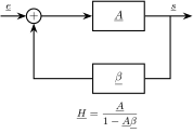
An amplifier of transfer function $\underline A(\jmath\omega)$ receives the input $\underline e$ plus a fraction $\underline\beta(\jmath\omega)\,\underline s$ of its own output $\underline s$ (positive feedback; for negative feedback change the sign of $\beta$ ). The closed-loop transfer function and the loop gain are

\underline H = \frac{\underline s}{\underline e} = \frac{\underline A}{1 - \underline A\,\underline\beta} , \qquad \underline T = \underline A\,\underline\beta .

Theorem 9.2 (Stability of a linear loop; oscillation condition)

Replacing $\jmath\omega$ by the complex variable $p$ , the free evolution of the loop is governed by the roots of its characteristic equation $1 - \underline A(p)\underline\beta(p) = 0$ (the poles of $\underline H$ ): each root $p_i$ contributes a mode $\eu^{p_it}$ . The loop is stable when all roots have negative real parts (every mode dies out); it oscillates, with growing amplitude, when a root has a positive real part. The frontier — a pair of purely imaginary roots $\pm\jmath \omega_0$ , i.e. a sustained sinusoid — is reached when

\underline A(\jmath\omega_0)\,\underline\beta(\jmath\omega_0) = 1

(Barkhausen’s condition: loop gain of modulus one and phase zero at $\omega_0$ ). For a second-order denominator $ap^2 + bp + c$ the loop is stable iff $a$ , $b$ , $c$ have the same sign.

Proof. The differential equation of the loop is obtained from $\underline s(1 - \underline A\underline\beta) = \underline A\underline e$ by reading each power of $\jmath\omega$ as a time derivative; its homogeneous solutions are the $\eu^{p_it}$ with $p_i$ the roots of the polynomial. Growth or decay follows the sign of $\operatorname{Re}p_i$ ; for a second-order polynomial the roots have negative real parts exactly when the coefficients share one sign (their sum is $-b/a$ and their product $c/a$ ). Barkhausen’s condition is the existence of a root at $p = \jmath\omega_0$ . ∎

Remark 9.3 (How an oscillator starts and stops)

An oscillator is designed with a loop gain slightly larger than one at $\omega_0$ : the noise present at switch-on contains that frequency, which grows exponentially while all others die. Linear theory then predicts infinite amplitude; in reality some non-linearity — the saturation of the amplifier, or a deliberately non-linear element — lowers the effective gain as the amplitude grows, until the loop gain averages exactly one: the amplitude settles. Every real oscillator is thus a linear loop for the frequency and a non-linear one for the amplitude; the gentler the limiting, the purer the sine wave.

9.2 The Wien-bridge oscillator

Proposition 9.4 (Wien-bridge oscillator)

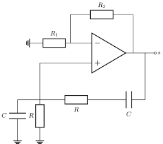
An op-amp in the non-inverting configuration of gain $K = 1 + R_2/R_1$ feeds its output back to its $+$ input through the Wien network: $R$ and $C$ in series, then $R$ and $C$ in parallel to ground. The network’s transfer function is

\underline\beta(\jmath\omega) = \frac1{3 + \jmath(RC\omega - 1/RC\omega)} ,

real and maximal ( $= 1/3$ ) at $\omega_0 = 1/RC$ . The loop gain $K\underline\beta$ equals one at $\omega_0$ when $K = 3$ : the circuit then sustains a sinusoid at

f_0 = \frac1{2\pi RC} .

The voltage $v$ at the $+$ input obeys

\frac{\dd^2v}{\dd t^2} + \frac{3 - K}{RC}\,\frac{\dd v}{\dd t} + \frac{v}{R^2C^2} = 0 :

for $K < 3$ the oscillation dies, for $K > 3$ it grows (negative damping) with the time constant $2RC/(K - 3)$ , until the op-amp’s saturation limits it.

Proof. Voltage divider: the series branch $Z_s = R + 1/\jmath C\omega$ , the parallel branch $Z_p = R/(1 + \jmath RC\omega)$ ; $\underline\beta = Z_p/(Z_s + Z_p)$ , which simplifies to the form given. Loop: $\underline v = \underline\beta K\underline v$ , i.e. $[3 + \jmath(RC\omega - 1/RC\omega)]\underline v = K\underline v$ ; multiply by $\jmath\omega RC$ and read $\jmath\omega \to \dd/\dd t$ : $R^2C^2\ddot v + (3 - K)RC\dot v + v = 0$ . Its damping coefficient changes sign at $K = 3$ . ∎

Left: a feedback loop — the output is fed back, through , to the input of the amplifier. Right: the Wien-bridge oscillator — a non-inverting amplifier of gain 1 + R_2/R_1 whose output returns to its + input through the series–parallel RC network; it oscillates at 1/2π RC when the gain reaches 3. — Left: a feedback loop — the output is fed back, through $\underline\beta$ , to the input of the amplifier. Right: the Wien-bridge oscillator — a non-inverting amplifier of gain $1 + R_2/R_1$ whose output returns to its $+$ input through the series–parallel $RC$ network; it oscillates at $1/2\pi RC$ when the gain reaches 3.

Example 9.5 (A 1 kHz source)

$R = 15.9\,\mathrm{k}\Omega$ , $C = 10\,\mathrm{nF}$ : $f_0 = 1.00\,\mathrm{kHz}$ . With $R_1 = 10\,\mathrm{k}\Omega$ and $R_2 = 21\,\mathrm{k}\Omega$ , $K = 3.1$ : the amplitude grows by $\eu$ every $2RC/0.1 = 3.2\,\mathrm{ms}$ from the switch-on noise, reaching saturation in a few tens of milliseconds; the clipped sine is then rich in harmonics. Replacing $R_1$ by a small incandescent lamp, whose resistance rises as it warms, pulls $K$ down to exactly $3$ at a moderate amplitude: a sine wave with less than $0.1\%$ of distortion, the circuit of the first laboratory signal generators.

9.3 Comparators with hysteresis; the astable multivibrator

Proposition 9.6 (Hysteresis comparator)

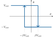
An op-amp with positive feedback — output fed to the $+$ input through a divider $R_1$ , $R_2$ (the $+$ input then sits at $\beta s$ with $\beta = R_1/(R_1 + R_2)$ when the signal $e$ is applied to the $-$ input) — has no stable linear regime: its output sits at $+V_{\text{sat}}$ or $-V_{\text{sat}}$ and switches

\begin{align*} &\text{from } +V_{\text{sat}} \text{ to } -V_{\text{sat}} \text{ when } e \text{ rises above } +\beta V_{\text{sat}} ,\\ &\text{from } -V_{\text{sat}} \text{ to } +V_{\text{sat}} \text{ when } e \text{ falls below } -\beta V_{\text{sat}} . \end{align*}

The two thresholds differ: the hysteresis $2\beta V_{\text{sat}}$ makes the comparator immune to noise smaller than that, and its cycle in the $(e, s)$ plane is a rectangle run clockwise.

Proof. With $s = +V_{\text{sat}}$ the $+$ input is at $+\beta V_{\text{sat}}$ ; the output stays positive as long as $e < \beta V_{\text{sat}}$ , and flips when $e$ crosses it — after which the $+$ input is at $-\beta V_{\text{sat}}$ , so $e$ must fall below that to flip it back. (In the linear regime the positive feedback would make any deviation grow: it is unstable.) ∎

Proposition 9.7 (Astable multivibrator)

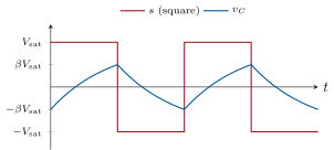
Feed the output of the hysteresis comparator back to its own $-$ input through an $RC$ circuit ( $R$ from $s$ to the $-$ input, $C$ from there to ground). The capacitor charges toward $\pm V_{\text{sat}}$ and flips the comparator each time it reaches a threshold: a square wave at $s$ , a near-triangular wave on $C$ , with the period

T = 2RC\,\ln\frac{1 + \beta}{1 - \beta} .

For $\beta = 1/2$ , $T = 2RC\ln3 \approx 2.2RC$ . Such relaxation oscillators clock microcontrollers, blink indicators and generate the triangle and square waves of function generators.

Proof. With $s = +V_{\text{sat}}$ , the capacitor voltage $v_C$ goes from $-\beta V_{\text{sat}}$ toward $+V_{\text{sat}}$ as $v_C = V_{\text{sat}} - (1 + \beta) V_{\text{sat}}\eu^{-t/RC}$ , and reaches $+\beta V_{\text{sat}}$ after $RC\ln[(1 + \beta) /(1 - \beta)]$ ; the comparator flips and the symmetric half-cycle follows. ∎

Left: the cycle of a hysteresis comparator — two thresholds, a rectangle run clockwise. Right: the astable multivibrator — the capacitor voltage shuttles between the thresholds and the output is a square wave.

9.4 Sampling a signal

Theorem 9.8 (Sampling; the Nyquist–Shannon criterion)

A signal is sampled when only its values $s(nT_s)$ at the instants $nT_s$ are kept, $f_s = 1/T_s$ being the sampling rate. The spectrum of the sampled signal is the spectrum of $s$ repeated around every multiple of $f_s$ . A signal whose spectrum is confined below $f_{\max}$ can be exactly reconstructed from its samples if and only if

f_s > 2f_{\max} ;

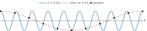
otherwise the copies overlap and a component at $f > f_s/2$ reappears at the alias frequency $|f - nf_s|$ (for the integer $n$ that brings it below $f_s/2$ ), indistinguishable from a true low-frequency component. Hence the anti-aliasing filter placed before any sampler: a low-pass that removes everything above $f_s/2$ .

Proof. Sampling is multiplying $s(t)$ by a periodic train of narrow pulses of period $T_s$ , whose Fourier series contains all the harmonics $nf_s$ (the mathematics volume of this year); multiplying $s$ by $\cos(2\pi nf_st)$ shifts its spectrum by $\pm nf_s$ — whence the copies. They do not overlap iff $f_{\max} < f_s - f_{\max}$ ; a low-pass of cut-off $f_s/2$ then recovers the original spectrum exactly (admitted). Aliasing: the samples of $\cos(2\pi ft)$ and of $\cos(2\pi(f - nf_s)t)$ at $t = mT_s$ coincide, since $2\pi nf_smT_s = 2\pi nm$ . ∎

Example 9.9 (Wagon wheels, CDs and oscilloscopes)

A film at $24$ images per second samples the world at $24\,\mathrm{Hz}$ : a wheel with $12$ spokes turning at $2.1$ turns per second presents a spoke $25.2$ times a second, $1.2$ beyond $f_s$ — it seems to turn slowly forward, and backward at $1.9$ turns per second. A compact disc samples at $44.1\,\mathrm{kHz}$ to reproduce sound up to $20\,\mathrm{kHz}$ , with a steep anti-aliasing filter between $20$ and $22\,\mathrm{kHz}$ . A digital oscilloscope set to $1\,\mathrm{MS}/\mathrm{s}$ displays a $999\,\mathrm{kHz}$ sine as a $1\,\mathrm{kHz}$ one — the first trap of digital measurement.

Aliasing: a sinusoid at 0.9f_s and one at 0.1f_s pass through the same samples; once sampled, they cannot be told apart — hence the criterion f_s > 2f_. — Aliasing: a sinusoid at $0.9f_s$ and one at $0.1f_s$ pass through the same samples; once sampled, they cannot be told apart — hence the criterion $f_s > 2f_{\max}$ .

Remark 9.10 (Quantization)

The analog-to-digital converter also rounds each sample to one of $2^N$ levels ( $N$ bits): the rounding error, at most half a step, acts as a noise of rms value $\Delta/\sqrt{12}$ for a step $\Delta$ , and the dynamic range (largest sine over that noise) is about $6N + 2$ dB — $98\,\mathrm{dB}$ for the $16$ bits of a CD, $74\,\mathrm{dB}$ for a $12$ -bit oscilloscope. Sampling rate and resolution are the two numbers on the label of every digitizer.

9.5 Synchronous detection

Proposition 9.11 (Synchronous (lock-in) detection)

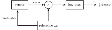
A signal of known frequency, $s(t) = A\cos(\omega_0t + \varphi)$ , buried in a noise $n(t)$ of much larger amplitude spread over a wide band, is multiplied by a reference $r(t) = \cos\omega_0t$ of the same frequency and passed through a low-pass filter of cut-off $f_c \ll f_0$ :

s(t)r(t) = \tfrac12A\cos\varphi + \tfrac12A\cos(2\omega_0t + \varphi) \ \xrightarrow{\ \text{low-pass}\ }\ \tfrac12A\cos\varphi .

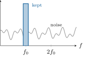
The output is a DC voltage proportional to the signal’s amplitude (and to the cosine of its phase relative to the reference), while the noise is reduced to the part of its spectrum lying within $\pm f_c$ of $f_0$ — a bandwidth $2f_c$ that can be made arbitrarily narrow (a fraction of a hertz for a filter time constant of seconds). Components at other frequencies $f$ are shifted to $f \pm f_0$ and rejected by the filter.

Proof. $\cos a\cos b = \tfrac12[\cos(a - b) + \cos(a + b)]$ ; the filter keeps the difference term for the signal, the $2\omega_0$ term and every noise component at $f$ being shifted to $|f - f_0|$ and $f + f_0$ — only the noise originally within $f_c$ of $f_0$ lands below $f_c$ . ∎

Synchronous detection: the sensor’s output, signal plus broad noise, is multiplied by a reference at the signal’s own frequency and low-pass filtered; only the noise within a narrow band around f_0 (shaded) survives, and the signal comes out as a DC level. — Synchronous detection: the sensor’s output, signal plus broad noise, is multiplied by a reference at the signal’s own frequency and low-pass filtered; only the noise within a narrow band around $f_0$ (shaded) survives, and the signal comes out as a DC level.

Example 9.12 (Finding a microvolt)

A photodiode delivers $10\,\text{µ}\mathrm{V}$ of signal when its light is chopped at $1\,\mathrm{kHz}$ , on top of $50\,\mathrm{nV}/\sqrt{\mathrm{Hz}}$ of white noise over $100\,\mathrm{kHz}$ ( $16\,\text{µ}\mathrm{V}$ rms: more than the signal). After synchronous detection with a filter of time constant $\tau = 1\,\mathrm{s}$ (noise bandwidth $1/4\tau = 0.25\,\mathrm{Hz}$ ) the noise is $50\,\text{nV} \times \sqrt{0.25} = 25\,\mathrm{nV}$ : a signal-to-noise ratio of $400$ — at the price of waiting a few seconds per point. The same trick, under the name of demodulation, recovers the music from an AM radio carrier and the data from a modem.

Method 9.13 (Designing a measurement chain)

(1) Modulate the quantity to be measured at a frequency $f_0$ away from the noise (chopper, AC bridge). (2) Amplify with a bandwidth covering $f_0$ . (3) Detect synchronously with a filter whose time constant is the longest the measurement can afford: the noise falls as $1/\sqrt\tau$ . (4) Sample the slow output at a rate above twice its bandwidth, after an anti-aliasing filter, with enough bits for the required resolution. (5) Check the chain with a known signal, and that nothing in it oscillates: every amplifier with feedback is a potential oscillator.

9.6 Exercises

Exercise 9.1 ★

A Wien-bridge oscillator with $R = 10\,\mathrm{k}\Omega$ , $C = 10\,\mathrm{nF}$ : frequency; gain needed; values of $R_1$ , $R_2$ for $K = 3.05$ with $R_1 = 10\,\mathrm{k}\Omega$ ; time constant of the amplitude growth. Which components fix the frequency, which the start-up?

Solution

Solution of Exercise 9.1.

$f_0 = 1/2\pi RC = 1.59\,\mathrm{kHz}$ ; $K = 3$ ; $R_2 = 2.05R_1 = 20.5\,\mathrm{k}\Omega$ ; $\tau = 2RC/(K - 3) = 4\,\mathrm{ms}$ . $R$ , $C$ set the frequency; $R_1$ , $R_2$ the start-up (and the amplitude limiting).

Exercise 9.2 ★

Hysteresis comparator with $V_{\text{sat}} = \pm 13\,\mathrm{V}$ , $R_1 = 1.0\,\mathrm{k}\Omega$ , $R_2 = 4.0\,\mathrm{k}\Omega$ : thresholds, hysteresis width. A noisy signal crossing zero with $2\,\mathrm{V}$ of noise: how many times does the output switch per crossing, with and without hysteresis?

Solution

Solution of Exercise 9.2.

$\beta = 0.2$ : thresholds $\pm2.6\,\mathrm{V}$ , hysteresis $5.2\,\mathrm{V}$ . Noise of $2\,\mathrm{V}$ cannot re-cross a threshold $5.2\,\mathrm{V}$ away: one switch per crossing; without hysteresis the output chatters many times.

Exercise 9.3 ★

Astable multivibrator with $R = 10\,\mathrm{k}\Omega$ , $C = 100\,\mathrm{nF}$ , $\beta = 0.5$ : period and frequency; $R$ for $1.0\,\mathrm{kHz}$ ; amplitude of the triangular wave on the capacitor; what happens to $T$ if $\beta$ is raised to $0.9$ ?

Solution

Solution of Exercise 9.3.

$T = 2RC\ln3 = 2.2\,\mathrm{ms}$ , $455\,\mathrm{Hz}$ ; $R = 4.55\,\mathrm{k}\Omega$ for $1\,\mathrm{kHz}$ ; triangle between $\pm\beta V_{\text{sat}}$ ; $\beta = 0.9$ : $T = 2RC\ln19 = 5.9\,\mathrm{ms}$ , $2.7$ times longer.

Exercise 9.4 ★

(a) A CD samples at $44.1\,\mathrm{kHz}$ : maximum frequency reproduced. (b) A $30\,\mathrm{kHz}$ ultrasound leaks into the recording: at what frequency does it appear? (c) A wheel with $8$ spokes filmed at $25\,\mathrm{images}/\mathrm{s}$ turns at $3.2$ turns/s: apparent motion. (d) An oscilloscope at $10\,\mathrm{MS}/\mathrm{s}$ shows a clean $100\,\mathrm{kHz}$ sine; the true signal could be what other frequencies?

Solution

Solution of Exercise 9.4.

(a) $22.05\,\mathrm{kHz}$ . (b) $|30 - 44.1| = 14.1\,\mathrm{kHz}$ . (c) Spokes at $8 \times 3.2 = 25.6\,\mathrm{Hz}$ , alias $0.6\,\mathrm{Hz}$ : the wheel seems to creep forward at $0.075$ turn/s. (d) $100\,\mathrm{kHz} + n \times 10\,\mathrm{MHz}$ , or $n \times 10\,\mathrm{MHz} - 100\,\mathrm{kHz}$ : $9.9$ , $10.1$ , $19.9$ , $20.1\,\mathrm{MHz}$ , …

Exercise 9.5 ★★

Loops with characteristic polynomials (a) $p^2 + 3p + 2$ , (b) $p^2 - p + 4$ , (c) $p^2 + 4$ , (d) $p^3 + 2p^2 + 2p + 1$ , (e) $p^3 + p + 1$ : find or discuss the roots; which loops are stable, which oscillate, which grow? (For the cubics, reason on the sign of the real parts: e.g. show (e) has a real negative root and two complex roots with positive real part, using the product and sum of the roots.)

Solution

Solution of Exercise 9.5.

(a) $-1$ , $-2$ : stable. (b) $(1 \pm \iu\sqrt{15})/2$ : growing oscillation. (c) $\pm2\iu$ : sustained oscillation. (d) $(p + 1)(p^2 + p + 1)$ : $-1$ and $(-1 \pm \iu\sqrt3)/2$ : stable. (e) One real root near $-0.68$ (the polynomial is monotonic); the sum of the three roots is $0$ , so the complex pair has real part $+0.34$ : unstable.

Exercise 9.6 ★★

Wien network. (a) Derive $\underline\beta(\jmath\omega)$ from the divider. (b) Plot (sketch) its modulus and phase; show the phase is zero only at $\omega_0$ and that the modulus is then $1/3$ . (c) Write the differential equation of the loop for a gain $K$ and discuss $K < 3$ , $K = 3$ , $K > 3$ . (d) With $K = 3.2$ , starting from a $1\,\mathrm{mV}$ noise, how long until the amplitude reaches $10\,\mathrm{V}$ ? Why does the final amplitude not depend on the initial noise?

Solution

Solution of Exercise 9.6.

(a) $\underline\beta = Z_p/(Z_s + Z_p)$ with $Z_s = R + 1/\jmath C\omega$ , $Z_p = R/(1 + \jmath RC\omega)$ : $\underline\beta = 1/[3 + \jmath(RC\omega - 1/RC\omega)]$ . (b) Modulus $1/\sqrt{9 + (RC\omega - 1/RC\omega)^2}$ , maximal $1/3$ at $\omega_0$ ; phase $-\arctan [(RC\omega - 1/RC\omega)/3]$ , zero only at $\omega_0$ . (c) $R^2C^2\ddot v + (3 - K)RC \dot v + v = 0$ : damped, sustained, growing. (d) Growth time constant $2RC/0.2 = 10RC = 1.6\,\mathrm{ms}$ ; $\ln10^4 = 9.2$ constants: $15\,\mathrm{ms}$ . The final amplitude is set by the non-linearity (saturation), not by the seed, which only sets the delay.

Exercise 9.7 ★★

Triangle generator. An integrator (op-amp, $R$ , $C$ ) is fed by the square output $\pm V_{\text{sat}}$ of a hysteresis comparator whose input is the integrator’s output; the comparator thresholds are $\pm V_{\text{sat}}R_1/R_2$ . (a) Show the integrator output is a triangle; its slope. (b) Period $T = 4RCR_1/R_2$ . (c) Numbers: $R = 10\,\mathrm{k}\Omega$ , $C = 10\,\mathrm{nF}$ , $R_1/R_2 = 0.5$ . (d) Advantage over the simple astable for a function generator.

Solution

Solution of Exercise 9.7.

(a) The integrator’s output has slope $\mp V_{\text{sat}}/RC$ : a triangle. (b) Each ramp spans $2V_{\text{sat}}R_1/R_2$ at slope $V_{\text{sat}}/RC$ : $T = 4RCR_1/R_2$ . (c) $4 \times 10^{-4} \times 0.5 = 0.2\,\mathrm{ms}$ , $5\,\mathrm{kHz}$ . (d) An exactly linear triangle, a frequency proportional to $1/R$ (easy to sweep), square and triangle outputs from one circuit.

Exercise 9.8 ★★

Quantization. (a) A $16$ -bit converter on $\pm1\,\mathrm{V}$ : step, rms quantization noise, dynamic range in dB. (b) $12$ bits at $1\,\mathrm{MS}/\mathrm{s}$ : bit rate; same for $8$ bits at $1\,\mathrm{GS}/\mathrm{s}$ (a fast oscilloscope). (c) A $1\,\mathrm{mV}$ signal on the $16$ -bit converter: how many steps? What to do before the converter? (d) Why does a good audio system dither (add a little noise) before quantizing?

Solution

Solution of Exercise 9.8.

(a) $\Delta = 2/65536 = 30.5\,\text{µ}\mathrm{V}$ , noise $\Delta/\sqrt{12} = 8.8\,\text{µ}\mathrm{V}$ , $98\,\mathrm{dB}$ . (b) $12\,\mathrm{Mbit}/\mathrm{s}$ ; $8\,\mathrm{Gbit}/\mathrm{s}$ . (c) $33$ steps: amplify by $100$ or more first. (d) Dither turns the rounding error, correlated with the signal (distortion), into a harmless uncorrelated noise.

Exercise 9.9 ★★

A signal contains $1.0\,\mathrm{kHz}$ and $9.0\,\mathrm{kHz}$ components and is sampled at $10\,\mathrm{kS}/\mathrm{s}$ . (a) Where does each appear? (b) An anti-aliasing first-order $RC$ filter with $f_c = 2\,\mathrm{kHz}$ is added: attenuation at $9\,\mathrm{kHz}$ in dB; enough if $40\,\mathrm{dB}$ is wanted? (c) Order of the filter needed (attenuation $\approx 20n$ dB per decade); or, alternatively, sampling rate needed with the first-order filter. (d) Why do modern converters oversample and filter digitally?

Solution

Solution of Exercise 9.9.

(a) Both at $1\,\mathrm{kHz}$ . (b) $|H| = 1/\sqrt{1 + 4.5^2} = 0.22$ , $-13\,\mathrm{dB}$ : no. (c) $13\,\mathrm{dB} \times n \ge 40$ : third or fourth order; or a sampling rate such that the first-order filter gives $40\,\mathrm{dB}$ at $f_s - 1\,\mathrm{kHz}$ , i.e. at $100f_c = 200\,\mathrm{kHz}$ : $f_s \approx 400\,\mathrm{kS}/\mathrm{s}$ . (d) Oversampling pushes the alias band far up, where a gentle analog filter suffices; the sharp filtering is then done digitally before decimation.

Exercise 9.10 ★★★

Lock-in. Input $A\cos(\omega_0t + \varphi) + n(t)$ multiplied by $\cos\omega_0t$ and filtered by a first-order low-pass of time constant $\tau$ . (a) DC output. (b) Show that a noise component at $f = f_0 + \delta f$ gives, after the filter, an amplitude reduced by $1/\sqrt{1 + (2\pi\delta f\tau)^2}$ ; deduce the equivalent noise bandwidth $B = 1/4\tau$ (admit $\int_0^\infty \dd x/(1 + x^2) = \pi/2$ ). (c) A $1\,\text{µ}\mathrm{V}$ signal in $1\,\mathrm{mV}$ rms of white noise over $10\,\mathrm{kHz}$ : noise density; $\tau$ for a signal-to-noise ratio of $10$ ; measuring time. (d) A $50\,\mathrm{Hz}$ pickup of $1\,\mathrm{mV}$ pollutes the input, with $f_0 = 1\,\mathrm{kHz}$ : where does it go, and by how much is it attenuated for $\tau = 1\,\mathrm{s}$ ?

Solution

Solution of Exercise 9.10.

(a) $\tfrac12A\cos\varphi$ . (b) The component at $f_0 + \delta f$ lands at $\delta f$ and passes the filter with $|H| = 1/\sqrt{1 + (2\pi\delta f\tau)^2}$ ; the power transmission integrates to $\int_0^\infty\dd f/(1 + (2\pi f\tau)^2) = 1/4\tau$ . (c) $e_n = 1\,\text{mV}/\sqrt{10^4} = 10\,\text{µ}\mathrm{V}/\sqrt{\mathrm{Hz}}$ ; $e_n\sqrt B = 0.1\,\text{µ}\mathrm{V}$ needs $B = 1 \times 10^{-4}\,\mathrm{Hz}$ , $\tau = 2500\,\mathrm{s}$ : an hour per point. (d) To $950$ and $1050\,\mathrm{Hz}$ , attenuated by $1/2\pi \times 950 \approx 1.7 \times 10^{-4}$ ( $-75\,\mathrm{dB}$ ).

Exercise 9.11 ★★★

Quartz. A quartz crystal behaves, near its resonance, as a series $L$ , $C$ , $r$ branch ( $L = 8000\,\mathrm{H}$ , $C = 3.0\,\mathrm{fF}$ , $r = 30\,\mathrm{k}\Omega$ ) in parallel with $C_0 = 1.5\,\mathrm{pF}$ . (a) Series resonance frequency and quality factor $Q = L\omega_0/r$ . (b) Why does an oscillator built around it hold its frequency to a part in $10^6$ while the Wien bridge drifts by percent (think of the phase slope $\dd\varphi/\dd\omega$ of the feedback network near resonance, $\sim 2Q/\omega_0$ )? (c) A watch crystal at $32\,768\,\mathrm{Hz}$ is divided by $2^{15}$ : result; its frequency varies as $-0.04\,\text{ppm}\,(T - 25{}^{\circ}\mathrm{C})^2$ : error per month at $5{}^{\circ}\mathrm{C}$ . (d) Why is $32\,768\,\mathrm{Hz}$ chosen and not $1\,\mathrm{MHz}$ ?

Solution

Solution of Exercise 9.11.

(a) $f_0 = 1/2\pi\sqrt{LC} = 32.5\,\mathrm{kHz}$ ; $Q = L\omega_0/r = 5.4 \times 10^{4}\,$ . (b) Near resonance the feedback phase turns by $2Q/\omega_0$ per unit $\omega$ : a parasitic phase shift $\delta\varphi$ moves the frequency by $\delta\omega/\omega_0 = \delta\varphi/2Q$ — $10^{-6}$ for $Q = 10^5$ , percent for $Q = 1/3$ . (c) $1\,\mathrm{Hz}$ ; $-0.04 \times 400 = -16\,\mathrm{ppm}$ : $16 \times 10^{-6} \times 2.6 \times 10^6 = 41\,\mathrm{s}$ slow per month. (d) Low frequency means low power in the dividing logic, $2^{15}$ divides exactly to $1\,\mathrm{Hz}$ , and the tiny tuning-fork crystal fits a watch.

Exercise 9.12 ★★★

Negative resistance. An op-amp has $R_2$ from output to $-$ input, $R_1$ from $-$ input to ground, and $R$ from output to $+$ input; the dipole seen between the $+$ input and ground is studied (linear regime). (a) Show that it behaves as a resistance $-RR_1/R_2$ . (b) This dipole is connected across a parallel $LC$ circuit of loss resistance $R_p$ (in parallel): write the equation of the voltage and find the condition for sustained oscillation and the frequency. (c) Numbers: $L = 10\,\mathrm{mH}$ , $C = 100\,\mathrm{nF}$ , $R_p = 50\,\mathrm{k}\Omega$ ; choose $R$ , $R_1 = R_2$ . (d) What limits the amplitude, and how does this oscillator compare with the Wien bridge?

Solution

Solution of Exercise 9.12.

(a) $v_- = v_+ = v$ , $v_{\text{out}} = v(1 + R_2/R_1)$ ; the current entering the dipole, $i = (v - v_{\text{out}})/R = -vR_2/RR_1$ : $v/i = -RR_1/R_2$ . (b) $C\dot v + v(1/R_p - R_2/RR_1) + \frac1L\int v\,\dd t = 0$ : sustained when $R = R_pR_2/R_1$ , at $\omega = 1/\sqrt{LC}$ (growing for smaller $R$ ). (c) $f = 5.0\,\mathrm{kHz}$ , $R \lesssim 50\,\mathrm{k}\Omega$ (say $48\,\mathrm{k}\Omega$ ). (d) Saturation; the tank’s $Q = R_p \sqrt{C/L} = 160$ gives a far steadier frequency than the Wien network.

9.7 Problem: A lock-in measurement chain

Problem 9.1

Weekend problem — from the reference oscillator to the digitized result: measuring ten microvolts of light signal under a millivolt of noise

A faint light is to be measured with a photodiode. The light is chopped by a rotating wheel at $f_0 = 1.00\,\mathrm{kHz}$ , so that the photodiode’s output is a sinusoid of amplitude $A = 10\,\text{µ}\mathrm{V}$ at $f_0$ (after a first amplifier), on which rides a white noise of spectral density $e_n = 50\,\mathrm{nV}/\sqrt{\mathrm{Hz}}$ over a bandwidth of $100\,\mathrm{kHz}$ , plus a $50\,\mathrm{Hz}$ mains pickup of $1.0\,\mathrm{mV}$ . The chopper’s own frequency is set by a Wien-bridge oscillator.

Part I — The reference oscillator. Wien bridge with $C = 10\,\mathrm{nF}$ , op-amp saturating at $\pm12\,\mathrm{V}$ .

$R$ for $f_0 = 1.00\,\mathrm{kHz}$ .
Derive the transfer function of the Wien network and check that its phase vanishes at $f_0$ with modulus $1/3$ .
Write the differential equation of the loop for a gain $K$ ; for $K = 3.15$ , time for the amplitude to grow by a factor $1000$ .
The amplitude is finally limited by saturation: describe the waveform, and why its harmonics matter for a reference.
A thermistor in place of $R_1$ (resistance falling when it warms) or a lamp (rising): which one stabilizes the gain at 3, and how?
The capacitors drift by $+1\%$ with temperature: new frequency. Why does the chopper then still work for the measurement (what must the reference do)?
The Wien network has a quality factor of about $1/3$ : what does that imply for the purity of the frequency compared with a quartz ( $Q \sim 10^5$ )?

Part II — The signal and the noise.

Rms value of the white noise over the full $100\,\mathrm{kHz}$ ; signal-to-noise ratio at the amplifier output.
A band-pass filter of quality factor $Q = 10$ centred on $f_0$ (noise bandwidth $\approx f_0/Q$ ) is inserted: noise rms and SNR. Why is this not sufficient for a precise measurement (think of drifts and of the $50\,\mathrm{Hz}$ )?
Why chop the light at $1\,\mathrm{kHz}$ instead of measuring the DC photocurrent directly? (Amplifiers have " $1/f$ " noise rising below a few hundred hertz.)
Signal amplitude if the chopper wheel produces a square modulation instead of a sine: which harmonic does the lock-in keep, and with what amplitude (Fourier coefficient $4/\pi$ for the fundamental of a square wave of unit amplitude)?
The photodiode also receives room light at $100\,\mathrm{Hz}$ (fluorescent tubes): what does the chain do with it?

Part III — Synchronous detection. The amplified signal is multiplied by the reference $\cos(2\pi f_0t)$ and filtered by a first-order low-pass of time constant $\tau$ .

Output of the multiplier for the signal alone (phase $\varphi$ between signal and reference); the DC term.
Attenuation of the $2f_0$ term by the filter for $\tau = 1\,\mathrm{s}$ (in dB).
Equivalent noise bandwidth $1/4\tau$ ; rms noise at the output for $\tau = 1\,\mathrm{s}$ and the SNR; same for $\tau = 10\,\mathrm{s}$ .
Where does the $50\,\mathrm{Hz}$ pickup end up, and with what attenuation for $\tau = 1\,\mathrm{s}$ ?
The phase $\varphi$ is unknown: what is lost if $\varphi = 60{}^{\circ}$ ? Describe the two-channel (in-phase and quadrature) lock-in and how it recovers $A$ whatever $\varphi$ .
Response time of the measurement (time to reach $99\%$ of the final value) for $\tau = 1\,\mathrm{s}$ ; the trade-off it expresses.
The reference drifts to $1001\,\mathrm{Hz}$ while the chopper stays at $1000\,\mathrm{Hz}$ : output of the lock-in; why the reference must be taken from the chopper itself.

Part IV — Digitizing.

The lock-in output is sampled by a computer: minimum rate for $\tau = 1\,\mathrm{s}$ (take the output bandwidth as $1/2\pi\tau$ ); a comfortable choice.
Alternatively the raw $1\,\mathrm{kHz}$ signal is digitized and the detection done in software: minimum sampling rate; the noise extends to $100\,\mathrm{kHz}$ — what must be done before sampling, and what attenuation at $100\,\mathrm{kHz}$ does a sampling at $20\,\mathrm{kS}/\mathrm{s}$ with a fourth-order filter cut at $5\,\mathrm{kHz}$ give ( $80\,\mathrm{dB}$ per decade)?
A $16$ -bit converter on $\pm1\,\mathrm{V}$ : step; the $10\,\text{µ}\mathrm{V}$ signal amplified by $1000$ : how many steps, and does the noise help or hurt?
Digital lock-in: the computer multiplies each sample by $\cos(2\pi f_0nT_s)$ and averages $N$ samples. At $20\,\mathrm{kS}/\mathrm{s}$ , $N$ for a $1\,\mathrm{s}$ average; by what factor is the white noise reduced, and is it the same as the analog filter’s?
A $1\,\mathrm{kHz}$ signal sampled at $999\,\mathrm{S}/\mathrm{s}$ : what does the computer see? How does this relate to the lock-in’s own principle?
Summarize the chain in a table: each stage, what it does to the signal, what it does to the noise.

Solution

Solution of Problem 9.1.

1. $R = 1/2\pi f_0C = 15.9\,\mathrm{k}\Omega$ .

2. $\underline\beta = 1/[3 + \jmath(RC\omega - 1/RC\omega)]$ : real, $= 1/3$ , at $\omega_0 = 1/RC$ .

3. $R^2C^2\ddot v + (3 - K)RC\dot v + v = 0$ ; time constant $2RC/0.15 = 2.1\,\mathrm{ms}$ ; $\ln1000 = 6.9$ : $15\,\mathrm{ms}$ .

4. A sine with flattened tops: odd harmonics. A reference rich in harmonics also detects the signal’s harmonics (and noise there): the result no longer measures the fundamental alone.

5. The lamp: as the amplitude rises it warms, $R_1$ rises and $K = 1 + R_2/R_1$ falls to $3$ . A thermistor in place of $R_1$ would do the opposite (it belongs in place of $R_2$ ).

6. $f \propto 1/C$ : $990\,\mathrm{Hz}$ . The lock-in reference is taken from the chopper itself (a detector on the wheel), so it follows.

7. $Q \sim 1/3$ : a small phase shift anywhere in the loop moves the frequency by percent; a quartz’s $10^5$ holds it to $10^{-6}$ .

8. $50\,\text{nV} \times \sqrt{10^5} = 16\,\text{µ}\mathrm{V}$ rms: SNR $0.6$ .

9. $B = 100\,\mathrm{Hz}$ : $0.5\,\text{µ}\mathrm{V}$ , SNR $20$ — but the filter’s centre drifts with its components, and the $50\,\mathrm{Hz}$ pickup is only attenuated by $\sim 1/[Q(f_0/f - f/f_0)] = 0.005$ : $5\,\text{µ}\mathrm{V}$ , half the signal.

10. Below a few hundred hertz the amplifier’s $1/f$ noise and drifts dominate; at $1\,\mathrm{kHz}$ the noise floor is white and low, and offsets do not count.

11. A square modulation between $0$ and $A_0$ is $A_0/2 + (2A_0/\pi) \cos\omega_0t + \dots$ : the lock-in keeps the fundamental, $0.64A_0$ .

12. $100\,\mathrm{Hz}$ is mixed to $900$ and $1100\,\mathrm{Hz}$ and removed by the low-pass.

13. $\tfrac12A\cos\varphi + \tfrac12A\cos(2\omega_0t + \varphi)$ ; DC term $\tfrac12A\cos\varphi$ .

14. $1/2\pi f\tau = 1/2\pi \times 2000 = 8 \times 10^{-5}$ : $-82\,\mathrm{dB}$ .

15. $B = 1/4\tau = 0.25\,\mathrm{Hz}$ : $e_n\sqrt B = 25\,\mathrm{nV}$ against $A = 10\,\text{µ}\mathrm{V}$ : SNR $400$ ; $\tau = 10\,\mathrm{s}$ : $7.9\,\mathrm{nV}$ , SNR $1300$ .

16. To $950$ and $1050\,\mathrm{Hz}$ : attenuated by $1/2\pi \times 950 = 1.7 \times 10^{-4}$ ( $-75\,\mathrm{dB}$ ): $0.17\,\text{µ}\mathrm{V}$ of ripple, a tenth of the signal — still worth a notch filter upstream.

17. $\cos60^\circ = 0.5$ : half the signal. A second multiplier with the reference shifted by $90{}^{\circ}$ gives $Y = \tfrac12A\sin\varphi$ ; with $X = \tfrac12A\cos\varphi$ , $A = 2\sqrt{X^2 + Y^2}$ and $\varphi = \arctan(Y/X)$ , whatever $\varphi$ .

18. $\tau\ln100 = 4.6\,\mathrm{s}$ ; the noise falls as $1/\sqrt\tau$ , the measurement time grows as $\tau$ .

19. The difference term is $\tfrac12A\cos(2\pi \times 1\,\text{Hz}\,t + \varphi)$ , passed by the filter with $1/\sqrt{1 + (2\pi)^2} = 0.16$ : a slow oscillation instead of a level. The reference must be coherent with the signal: take it from the chopper.

20. Bandwidth $1/2\pi\tau = 0.16\,\mathrm{Hz}$ : above $0.32\,\mathrm{S}/\mathrm{s}$ ; $10\,\mathrm{S}/\mathrm{s}$ is comfortable.

21. At least $2\,\mathrm{kS}/\mathrm{s}$ ; an anti-aliasing filter is mandatory; fourth order at $5\,\mathrm{kHz}$ : $80\log_{10}(100/5) = 104\,\mathrm{dB}$ at $100\,\mathrm{kHz}$ (and $46\,\mathrm{dB}$ at $19\,\mathrm{kHz}$ , the noise that would alias onto $1\,\mathrm{kHz}$ ).

22. Step $30.5\,\text{µ}\mathrm{V}$ ; $10\,\mathrm{mV}$ is $330$ steps; the amplified noise ( $16\,\mathrm{mV}$ rms) spans many steps and, averaged, lets the mean be resolved far below one step: it helps.

23. $N = 20000$ ; the white noise falls by $\sqrt N = 140$ ; a $1\,\mathrm{s}$ boxcar has a noise bandwidth $1/2T = 0.5\,\mathrm{Hz}$ — twice the analog $RC$ ’s, comparable.

24. The samples walk slowly through the sine: a $1\,\mathrm{Hz}$ alias. The lock-in does the same thing on purpose: sampling at the reference phase is multiplying by the reference.

25. Chopper: signal moved to $1\,\mathrm{kHz}$ , noise unchanged (but the $1/f$ part avoided). Amplifier: both $\times$ gain. Multiplier: signal to DC, noise spread. Low-pass: signal kept, noise cut to $1/4\tau$ . Sampler/ADC: signal digitized, aliases and quantization controlled by the filter and the bit count.

Terms defined in this chapter

Closed loop; loop gain

See all 393 terms in the glossary