University Physics — Year 2 · Bachelor Year 2

29The Boltzmann Factor

Climb a mountain and the air thins: at three thousand metres the pressure has dropped to $0.7\,\mathrm{bar}$ , at the top of Everest to a third of its sea-level value. Nothing confines the atmosphere from above; it is held by gravity and spread out by thermal agitation, and the compromise between the two is an exponential, $n \propto \eu^{-mgz/k_BT}$ — the ratio of the potential energy of a molecule to $k_BT$ decides how rare it is up there. The same exponential governs the fraction of atoms in an excited level, the number of molecules fast enough to escape a planet, the magnetisation of a paramagnet, the populations that a laser must invert, and the quanta that Planck’s law counts: it is the Boltzmann factor, the single most useful formula of statistical physics. This chapter motivates it with the atmosphere, states it in general, and draws from it, with nothing but sums and Gaussian integrals, the two-level system and its heat capacity, the equipartition of energy, the distribution of molecular speeds, and the Curie law of paramagnetism — with, on the way, the mean energy of a quantum oscillator, which is Planck’s formula.

From a summit, the haze of the lower atmosphere and the deep blue above: the air’s density falls by a factor every 8\, km — the Boltzmann factor of a molecule’s potential energy in the Earth’s gravity. — From a summit, the haze of the lower atmosphere and the deep blue above: the air’s density falls by a factor $\eu$ every $8\,\mathrm{km}$ — the Boltzmann factor of a molecule’s potential energy in the Earth’s gravity.

29.1 The isothermal atmosphere

Proposition 29.1 (Barometric law)

In an atmosphere of perfect gas (molecular mass $m$ ) at uniform temperature $T$ in the uniform gravity $g$ , the pressure and the number density fall exponentially with altitude:

P(z) = P_0\,\eu^{-z/H}, \qquad n(z) = n_0\,\eu^{-mgz/k_BT}, \qquad H = \frac{k_BT}{mg} ,

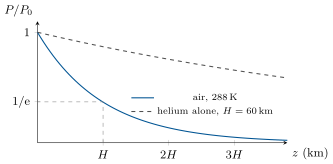
with the scale height $H \approx 8.4\,\mathrm{km}$ for air at $288\,\mathrm{K}$ . The exponent is the ratio of the potential energy $mgz$ of a molecule to the thermal energy $k_BT$ .

Proof. Hydrostatics, $\dd P/\dd z = -\rho g = -nmg$ , and the perfect-gas law $P = nk_BT$ : $\dd P/\dd z = -(mg/k_BT)P$ , an exponential. The real atmosphere cools with altitude (about $6.5\,\mathrm{K}/\mathrm{km}$ in the lowest ten kilometres), which makes the fall somewhat faster; the isothermal model is good to $20\%$ . ∎

$The isothermal atmosphere: pressure and density fall by 1/ every scale height H = k_BT/mg; a lighter gas would have a larger H — but below 100\, km turbulence keeps the air mixed, and all gases share the mean H.$

The isothermal atmosphere: pressure and density fall by

1/\eu

every scale height

H = k_BT/mg

; a lighter gas would have a larger

H

— but below

100\,\mathrm{km}

turbulence keeps the air mixed, and all gases share the mean

H

29.2 The Boltzmann factor

Theorem 29.2 (Boltzmann factor)

A system in thermal equilibrium with a thermostat at the temperature $T$ is found in a given microscopic state of energy $E$ with a probability proportional to

\eu^{-E/k_BT} .

Hence, for a set of discrete states of energies $E_i$ ,

p_i = \frac{\eu^{-E_i/k_BT}}{Z}, \qquad Z = \sum_i\eu^{-E_i/k_BT} ,

the sum $Z$ (the partition function) normalising the probabilities; two states (or two levels of equal degeneracy) are populated in the ratio $N_2/N_1 = \eu^{-(E_2 - E_1)/k_BT}$ ; and for a continuous variable (a position, a velocity) the probability density is proportional to $\eu^{-E/k_BT}$ in that variable. At $300\,\mathrm{K}$ , $k_BT = 4.1 \times 10^{-21}\,\mathrm{J} = 0.026\,\mathrm{eV}$ : anything that costs much more than this is rare, anything that costs much less is freely excited.

Proof. The barometric law is the factor for the potential energy $mgz$ ; we admit its generality, but here is the argument (made rigorous in the Year 3 volume). The thermostat $R$ is large; when our small system is in a state of energy $E$ , the thermostat has the energy $E_{\text{tot}} - E$ , and can be in $\Omega_R(E_{\text{tot}} - E)$ microscopic states, all equally probable (the fundamental postulate for an isolated whole). So $p(E) \propto \Omega_R(E_{\text{tot}} - E)$ . With Boltzmann’s definition of the entropy, $S_R = k_B\ln\Omega_R$ , and $1/T = \dd S_R/\dd E_R$ for the thermostat, $\ln\Omega_R(E_{\text{tot}} - E) \approx \ln\Omega_R(E_{\text{tot}}) - E/k_BT$ since $E \ll E_{\text{tot}}$ ; exponentiate. ∎

Example 29.3 (Populations of atomic levels)

Hydrogen’s first excited level lies $10.2\,\mathrm{eV}$ above the ground state: at $300\,\mathrm{K}$ , $\eu^{-395}$ — not one atom in the universe; at $6000\,\mathrm{K}$ , the Sun’s surface, $\eu^{-19.7} \approx 3 \times 10^{-9}$ (times a degeneracy of $4$ ): enough, in the Sun’s huge column of gas, for the Balmer absorption lines, which are strongest in stars near $10\,000\,\mathrm{K}$ . The sodium D line ( $2.1\,\mathrm{eV}$ ) in a $2500\,\mathrm{K}$ flame: $\eu^{-9.8} = 6 \times 10^{-5}$ of the atoms are excited, which gives the yellow flame of a pinch of salt. And the laser medium of Chapter 23: the factor says its upper level is empty at equilibrium, and the pump must fight it.

29.3 Discrete levels: the two-level system and the oscillator

Proposition 29.4 (Mean energy from the partition function)

With $\beta = 1/k_BT$ ,

\langle E\rangle = \sum_ip_iE_i = -\frac{\partial\ln Z}{\partial\beta}, \qquad C = \frac{\dd\langle E\rangle}{\dd T} .

Proof. $\partial_\beta Z = -\sum E_i\eu^{-\beta E_i}$ , divide by $Z$ . ∎

Proposition 29.5 (Two-level system)

$N$ independent systems with two levels $0$ and $\varepsilon$ (spins in a field, atoms with one excited level, defects with two positions):

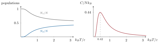
\frac{N_2}{N} = \frac{1}{\eu^{\varepsilon/k_BT} + 1}, \qquad \langle E\rangle = \frac{N\varepsilon}{\eu^{\varepsilon/k_BT} + 1}, \qquad C = Nk_B\,\frac{x^2\eu^x}{(\eu^x + 1)^2}, \quad x = \frac{\varepsilon}{k_BT} .

The upper level is empty at low temperature and at most half-filled at high temperature (never inverted at equilibrium); the heat capacity vanishes at both ends and peaks at $0.44\,Nk_B$ near $k_BT = 0.42 \varepsilon$ — the Schottky anomaly, the signature of a gap in the spectrum.

Proof. $Z = 1 + \eu^{-x}$ ; $p_2 = \eu^{-x}/(1 + \eu^{-x})$ ; differentiate $\langle E\rangle$ with respect to $T$ . ∎

The two-level system: populations against temperature (the upper level fills toward one half, never beyond) and the Schottky heat capacity, a bump where k_BT matches the gap. — The two-level system: populations against temperature (the upper level fills toward one half, never beyond) and the Schottky heat capacity, a bump where $k_BT$ matches the gap.

Proposition 29.6 (The quantum oscillator and Planck’s formula)

A harmonic oscillator of frequency $\nu$ has the levels $E_n = nh\nu$ (plus a constant); at temperature $T$ ,

Z = \frac{1}{1 - \eu^{-h\nu/k_BT}}, \qquad \langle E\rangle = \frac{h\nu}{\eu^{h\nu/k_BT} - 1} \ \longrightarrow\ \begin{cases} k_BT & (h\nu \ll k_BT), \\ h\nu\,\eu^{-h\nu/k_BT} & (h\nu \gg k_BT). \end{cases}

This is the mean energy of a mode of the radiation field that Planck’s law (Chapter 26) multiplies by the number of modes, and the mean energy of a vibration in a solid: at high temperature the classical $k_BT$ , at low temperature a frozen mode.

Proof. Geometric series, then $-\partial_\beta\ln Z$ . ∎

Example 29.7 (Heat capacity of solids)

Treat each atom of a solid as three oscillators of the same frequency $\nu$ (Einstein, 1907): $C = 3Nk_B\,x^2\eu^x/(\eu^x - 1)^2$ with $x = h\nu/k_BT$ . Above $\theta_{\text{E}} = h\nu/k_B$ , $C \to 3Nk_B = 3R$ per mole — the law of Dulong and Petit ( $25\,\mathrm{J}/\mathrm{mol}/\mathrm{K}$ ), obeyed by lead, copper, iron at room temperature; far below it, $C$ collapses. Diamond ( $\theta_{\text{E}} \approx 1300\,\mathrm{K}$ ) has only $6\,\mathrm{J}/\mathrm{mol}/\mathrm{K}$ at $300\,\mathrm{K}$ , which classical physics could not explain, and every solid’s heat capacity vanishes at low temperature — the first success of the quantum outside radiation.

29.4 Equipartition and Maxwell’s distribution

Theorem 29.8 (Equipartition of energy)

Every variable $q$ that enters the energy quadratically, $E = aq^2 + \dots$ , and ranges over all real values, contributes $\tfrac12k_BT$ to the mean energy at equilibrium:

\langle aq^2\rangle = \tfrac12k_BT .

A monatomic gas (three translations) has $U = \tfrac32Nk_BT$ and $C_V = \tfrac32R$ per mole; a diatomic gas adds two rotations, $C_V = \tfrac52R$ , and its vibration (two quadratic terms, but quantised with $h\nu \gg k_BT$ at room temperature) stays frozen until a few thousand kelvins.

Proof. The probability density in $q$ is $\propto\eu^{-aq^2/k_BT}$ , a Gaussian:

\langle aq^2\rangle = \frac{\int aq^2\,\eu^{-aq^2/k_BT}\,\dd q}{\int\eu^{-aq^2/k_BT}\,\dd q} = \tfrac12k_BT

(differentiate $\int\eu^{-\lambda q^2}\dd q = \sqrt{\pi/\lambda}$ with respect to $\lambda$ ). The result needs the continuum: when the levels are spaced by more than $k_BT$ the factor freezes the variable, as for the oscillator above. ∎

Theorem 29.9 (Maxwell’s distribution of speeds)

In a gas at $T$ , the velocity components are independent Gaussians of variance $k_BT/m$ , and the speed $v = |\vect v|$ has the probability density

f(v) = 4\pi\Big(\frac{m}{2\pi k_BT}\Big)^{3/2}v^2\,\eu^{-mv^2/2k_BT} ,

with the most probable, mean and root-mean-square speeds

v_{\text{p}} = \sqrt{\frac{2k_BT}{m}}, \qquad \langle v\rangle = \sqrt{\frac{8k_BT}{\pi m}}, \qquad v_{\text{rms}} = \sqrt{\frac{3k_BT}{m}} ,

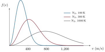
in the ratios $1 : 1.13 : 1.22$ . For nitrogen at $300\,\mathrm{K}$ : $422\,$ , $476\,$ , $517\,\mathrm{m}/\mathrm{s}$ ; for hydrogen, $3.7$ times more; the distribution’s tail, $\propto\eu^{-mv^2/2k_BT}$ , is what lets the fastest molecules evaporate, react, or leave a planet.

Proof. The kinetic energy $\tfrac12m(v_x^2 + v_y^2 + v_z^2)$ gives a factor $\eu^{-mv_x^2/2k_BT}\eu^{-mv_y^2/2k_BT}\eu^{-mv_z^2/2k_BT}$ : three independent Gaussians, each normalised by $\sqrt{m/2\pi k_BT}$ . The speed distribution collects all velocities in the shell of radius $v$ and volume $4\pi v^2\dd v$ . Then $v_{\text{p}}$ from $\dd f/\dd v = 0$ , and the moments from $\int_0^\infty v^3\eu^{-av^2}\dd v = 1/2a^2$ , $\int_0^\infty v^4\eu^{-av^2}\dd v = \tfrac38\sqrt{\pi/a^5}$ ; $v_{\text{rms}}$ also follows from equipartition, $\tfrac12m\langle v^2\rangle = \tfrac32k_BT$ . ∎

Maxwell’s speed distribution for nitrogen at three temperatures: the peak moves as √ T, the curve broadens, and the high-speed tail grows fastest of all — the tail that decides escape and reaction rates. — Maxwell’s speed distribution for nitrogen at three temperatures: the peak moves as $\sqrt T$ , the curve broadens, and the high-speed tail grows fastest of all — the tail that decides escape and reaction rates.

Example 29.10 (Who leaves the planet)

The Earth’s escape speed is $11.2\,\mathrm{km}/\mathrm{s}$ . In the exosphere, near $1000\,\mathrm{K}$ , helium has $v_{\text{p}} = 2.0\,\mathrm{km}/\mathrm{s}$ : the fraction of atoms above the escape speed is of order $\eu^{-(11.2/2.0)^2} = \eu^{-31} \approx 10^{-13}$ — small, but renewed at every collision for billions of years: helium leaks away, and its abundance in the air is only $5\,\mathrm{ppm}$ despite its constant production by radioactive decay. For nitrogen the exponent is seven times larger, $\eu^{-220}$ : nitrogen stays. On the Moon ( $v_{\text{esc}} = 2.4\,\mathrm{km}/\mathrm{s}$ ) even nitrogen at $400\,\mathrm{K}$ ( $v_{\text{p}} = 490\,\mathrm{m}/\mathrm{s}$ ) has $\eu^{-24}$ per collision time: over the age of the solar system, no atmosphere survives.

29.5 Paramagnetism and the Curie law

Proposition 29.11 (Spin-1/2 paramagnet)

$N$ independent magnetic moments that can only point along or against the field $B$ , with energies $\mp\mu B$ , have at temperature $T$ the mean moment and magnetisation

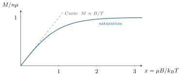
\langle\mu_z\rangle = \mu\tanh\frac{\mu B}{k_BT}, \qquad M = n\mu\tanh\frac{\mu B}{k_BT} \ \longrightarrow\ \begin{cases} n\mu^2B/k_BT & (\mu B \ll k_BT):\ \text{Curie's law}, \\ n\mu & (\mu B \gg k_BT):\ \text{saturation}. \end{cases}

The susceptibility $\chi = \mu_0M/B = \mu_0n\mu^2/k_BT$ varies as $1/T$ (Curie’s law); with $\mu = \mu_B = 9.27 \times 10^{-24}\,\mathrm{J}/\mathrm{T}$ , $\mu B/k_BT = 2.2 \times 10^{-3}$ at $1\,\mathrm{T}$ and $300\,\mathrm{K}$ , so ordinary paramagnets are barely magnetised; at $1\,\mathrm{K}$ the same field gives $0.67$ and the saturation begins.

Proof. $p_\pm \propto\eu^{\pm\mu B/k_BT}$ : $\langle\mu_z\rangle = \mu(\eu^x - \eu^{-x})/(\eu^x + \eu^{-x})$ with $x = \mu B/k_BT$ ; $\tanh x \approx x$ for small $x$ . ∎

Magnetisation of a spin-1/2 paramagnet: linear in B/T at small fields (Curie), saturating when B exceeds k_BT — reached at a tesla only below a kelvin, which makes the curve a thermometer for the coldest experiments. — Magnetisation of a spin-1/2 paramagnet: linear in $B/T$ at small fields (Curie), saturating when $\mu B$ exceeds $k_BT$ — reached at a tesla only below a kelvin, which makes the curve a thermometer for the coldest experiments.

Remark 29.12 (What the factor does not do)

The Boltzmann factor describes equilibrium at a temperature; it says nothing of rates (how fast the equilibrium is reached — though an activation energy $E_{\text{a}}$ gives rates $\propto\eu^{-E_{\text{a}}/k_BT}$ , the Arrhenius law met for diffusion in solids). It applies to independent subsystems or to the whole; for identical quantum particles at high density (electrons in a metal, photons, helium near absolute zero) it is replaced by the Fermi–Dirac and Bose–Einstein distributions of the Year 3 volume, of which it is the dilute limit.

Method 29.13 (Boltzmann estimates)

(1) Compute $E/k_BT$ ; $k_BT = 0.026\,\mathrm{eV}$ at $300\,\mathrm{K}$ , $1\,\mathrm{eV}$ at $11\,600\,\mathrm{K}$ . (2) Ratios of populations: $\eu^{-\Delta E/k_BT}$ (times degeneracies). (3) Discrete levels: $Z$ , then $\langle E\rangle = -\partial_\beta\ln Z$ , then $C$ . (4) Quadratic continuous variables: $\tfrac12k_BT$ each, if not frozen. (5) Speeds: $v_{\text{p}} = \sqrt{2k_BT/m}$ and the Gaussian tail. (6) Spins: $\tanh(\mu B/k_BT)$ , Curie’s $1/T$ .

29.6 Exercises

Exercise 29.1 ★

Scale height of air at $288\,\mathrm{K}$ ( $M = 29\,\mathrm{g}/\mathrm{mol}$ ); pressure at $3000\,\mathrm{m}$ , at $8849\,\mathrm{m}$ , at $10\,\mathrm{km}$ (compare with the measured $0.26\,\mathrm{bar}$ ); scale height of helium alone; of the Martian atmosphere (CO $_2$ , $210\,\mathrm{K}$ , $g = 3.7\,\mathrm{m}/\mathrm{s}^{2}$ ).

Solution

Solution of Exercise 29.1.

$H = k_BT/mg = 8.4\,\mathrm{km}$ ; $0.70\,$ , $0.35\,$ , $0.30\,\mathrm{bar}$ (the real $0.26\,$ : the air cools with height); helium $61\,\mathrm{km}$ ; Mars $10.7\,\mathrm{km}$ .

Exercise 29.2 ★

Populations: hydrogen’s $n = 2$ level ( $10.2\,\mathrm{eV}$ , degeneracy $4$ against $1$ ) at $300\,\mathrm{K}$ , $6000\,\mathrm{K}$ , $10\,000\,\mathrm{K}$ ; sodium’s $2.1\,\mathrm{eV}$ level in a $2500\,\mathrm{K}$ flame; a molecular rotation level at $1 \times 10^{-3}\,\mathrm{eV}$ at $300\,\mathrm{K}$ ; a nuclear spin level split by $1 \times 10^{-7}\,\mathrm{eV}$ in a magnet at $300\,\mathrm{K}$ .

Solution

Solution of Exercise 29.2.

Hydrogen: $4\eu^{-395} \approx 10^{-171}$ ; $4\eu^{-19.7} = 10^{-8}$ ; $4\eu^{-11.8} = 3 \times 10^{-5}$ . Sodium: $\eu^{-9.8} = 6 \times 10^{-5}$ . Rotation: $\eu^{-0.04} = 0.96$ , almost equal. Nuclear spin: $1 - 4 \times 10^{-6}$ — the tiny polarisation that magnetic resonance works with.

Exercise 29.3 ★

Maxwell speeds ( $v_{\text{p}}$ , $\langle v\rangle$ , $v_{\text{rms}}$ ) for N $_2$ at $300\,\mathrm{K}$ and $77\,\mathrm{K}$ , H $_2$ at $300\,\mathrm{K}$ , and for a smoke particle of $1 \times 10^{-18}\,\mathrm{kg}$ . Fraction of molecules faster than $2v_{\text{p}}$ (about $4.6\%$ ) and than $3v_{\text{p}}$ (about $4 \times 10^{-4}$ ): comment on the tail.

Solution

Solution of Exercise 29.3.

N $_2$ $300\,\mathrm{K}$ : $422\,$ , $476\,$ , $517\,\mathrm{m}/\mathrm{s}$ ; $77\,\mathrm{K}$ : $214\,$ , $241\,$ , $262\,\mathrm{m}/\mathrm{s}$ ; H $_2$ : $1580\,$ , $1780\,$ , $1930\,\mathrm{m}/\mathrm{s}$ ; smoke particle: $9\,\mathrm{cm}/\mathrm{s}$ (its Brownian shiver). Above $2v_{\text{p}}$ one molecule in twenty; above $3v_{\text{p}}$ one in $2500$ — still $10^{22}$ per cubic metre.

Exercise 29.4 ★

Spin-1/2 moments $\mu = \mu_B$ , $n = 1 \times 10^{28}\,\mathrm{m}^{-3}$ , $B = 1\,\mathrm{T}$ : $x = \mu B/k_BT$ at $300\,\mathrm{K}$ and $1\,\mathrm{K}$ ; $M/M_{\text{sat}}$ ; $M_{\text{sat}}$ ; the susceptibility at $300\,\mathrm{K}$ . Compare with iron’s saturation magnetisation ( $1.7 \times 10^{6}\,\mathrm{A}/\mathrm{m}$ ).

Solution

Solution of Exercise 29.4.

$x = 2.2 \times 10^{-3}$ and $0.67$ ; $M/M_{\text{sat}} = 2.2 \times 10^{-3}$ and $0.59$ ; $M_{\text{sat}} = n\mu = 9.3 \times 10^{4}\,\mathrm{A}/\mathrm{m}$ ; $\chi = \mu_0n\mu^2/k_BT = 2.6 \times 10^{-4}$ . Iron’s $1.7 \times 10^{6}\,\mathrm{A}/\mathrm{m}$ is cooperative, not a Boltzmann effect.

Exercise 29.5 ★★

Two levels. (a) Derive $p_1$ , $p_2$ , $\langle E\rangle$ from $Z$ . (b) Show that $N_2 < N_1$ at every positive temperature; what would $N_2 > N_1$ mean for $T$ ? (c) Entropy $S = -Nk_B\sum p_i\ln p_i$ of the system at $T \to 0$ and $T \to \infty$ . (d) A defect in a crystal can sit in two positions $0.05\,\mathrm{eV}$ apart: occupation of the upper one at $300\,\mathrm{K}$ and at $77\,\mathrm{K}$ .

Solution

Solution of Exercise 29.5.

(a) Proposition 29.5. (b) $\eu^{-x} < 1$ for $T > 0$ ; $N_2 > N_1$ would need $T < 0$ — a population inversion. (c) $0$ and $Nk_B\ln 2$ . (d) $x = 1.93$ : $0.13$ ; at $77\,\mathrm{K}$ , $x = 7.5$ : $5 \times 10^{-4}$ .

Exercise 29.6 ★★

Schottky. (a) Derive $C(T)$ of the two-level system. (b) Locate its maximum numerically ( $x = 2.40$ ) and its value. (c) Limits at low and high $T$ , with their physical meaning. (d) Nuclear spins of copper in $1\,\mathrm{T}$ have $\varepsilon \approx 1 \times 10^{-7}\,\mathrm{eV}$ : at what temperature does their Schottky peak sit, and why does it matter for the coldest cryostats?

Solution

Solution of Exercise 29.6.

(a) Derivative of $N\varepsilon/(\eu^x + 1)$ . (b) $x = 2.40$ , $C = 0.44\,Nk_B$ . (c) $\propto x^2\eu^{-x} \to 0$ : frozen; $\propto 1/T^2 \to 0$ : both levels full, nothing left to absorb. (d) $k_BT = 0.42\varepsilon$ : $0.5\,\mathrm{mK}$ ; below a millikelvin the nuclear spins hold most of the heat capacity and slow every cooling.

Exercise 29.7 ★★

Equipartition and its failure. (a) Derive $\langle aq^2\rangle = k_BT/2$ with the Gaussian integral. (b) $C_V$ of a monatomic and of a rigid diatomic gas. (c) Nitrogen’s vibration has $h\nu/k_B = 3400\,\mathrm{K}$ : using the oscillator’s mean energy, $C_V$ at $300\,\mathrm{K}$ , $1000\,\mathrm{K}$ , $3000\,\mathrm{K}$ . (d) Einstein solid: $C$ at $T = \theta_{\text{E}}$ , $\theta_{\text{E}}/4$ , $4\theta_{\text{E}}$ in units of $3R$ ; diamond at room temperature.

Solution

Solution of Exercise 29.7.

(a) Theorem 29.8. (b) $\tfrac32R$ , $\tfrac52R$ . (c) $C_{\text{vib}}/R = x^2\eu^x/(\eu^x - 1)^2$ : $0.002$ , $0.41$ , $0.90$ ; $C_V = 2.50R$ , $2.91R$ , $3.40R$ . (d) $0.92$ , $0.30$ , $0.995$ ; diamond $x = 4.3$ : $0.26 \times 3R = 6.5\,\mathrm{J}/\mathrm{mol}/\mathrm{K}$ .

Exercise 29.8 ★★

Maxwell in detail. (a) Show that the velocity components are independent Gaussians and derive $f(v)$ . (b) Compute $v_{\text{p}}$ , $\langle v\rangle$ , $v_{\text{rms}}$ . (c) Mean kinetic energy: check with equipartition. (d) The flux of molecules hitting a wall is $\tfrac14n\langle v\rangle$ per unit area and time (admitted): number of N $_2$ molecules hitting $1\,\mathrm{cm}^{2}$ per second at $1\,\mathrm{bar}$ , $300\,\mathrm{K}$ ; and the rate at which a $1\,\text{µ}\mathrm{m}$ pinhole lets air into a vacuum chamber (effusion).

Solution

Solution of Exercise 29.8.

(a), (b) Theorem 29.9. (c) $\tfrac32k_BT$ . (d) $\tfrac14n\langle v\rangle = 2.9 \times 10^{27}\,\mathrm{m}^{-2}\,\mathrm{s}^{-1}$ : $3 \times 10^{23}$ per square centimetre per second; through $7.9 \times 10^{-13}\,\mathrm{m}^{2}$ : $2.3 \times 10^{15}$ molecules per second, a leak of $1 \times 10^{-5}\,\mathrm{Pa}\,\mathrm{m}^{3}/\mathrm{s}$ .

Exercise 29.9 ★★

Escape. (a) Fraction of a Maxwell gas faster than $v$ : show it is approximately $(2/\sqrt\pi)\,x\,\eu^{-x^2}$ for $x = v/v_{\text{p}} \gg 1$ . (b) Helium at $1000\,\mathrm{K}$ above $11.2\,\mathrm{km}/\mathrm{s}$ ; nitrogen. (c) Moon, $v_{\text{esc}} = 2.4\,\mathrm{km}/\mathrm{s}$ , $400\,\mathrm{K}$ : nitrogen, and what temperature would hold it for the age of the solar system (take $10^{17}$ collision times: escape fraction below $10^{-17}$ ). (d) Why does Titan ( $2.6\,\mathrm{km}/\mathrm{s}$ , $94\,\mathrm{K}$ ) keep a thick nitrogen atmosphere?

Solution

Solution of Exercise 29.9.

(a) Integrate $f$ by parts; the leading term is $(2/\sqrt\pi)x\eu^{-x^2}$ . (b) Helium $x = 5.5$ : $5 \times 10^{-13}$ ; nitrogen $x = 14.5$ : $\eu^{-211}$ . (c) $x = 4.9$ : $10^{-10}$ per collision time — gone; $10^{-17}$ needs $x \approx 6.6$ , $T \lesssim 230\,\mathrm{K}$ . (d) $x = 11$ : $\eu^{-121}$ ; cold enough.

Exercise 29.10 ★★★

Other potentials. (a) In a centrifuge rotating at $\omega$ , the effective potential energy is $-\tfrac12m\omega^2r^2$ : density profile $n(r)$ . (b) Uranium hexafluoride, two isotopes $\Delta m = 3\,\mathrm{u}$ , $\omega = 2\pi \times 1000\,\mathrm{Hz}$ , $r = 10\,\mathrm{cm}$ , $300\,\mathrm{K}$ : enrichment factor of one stage. (c) Colloidal spheres (buoyant mass $m' = 2.6 \times 10^{-17}\,\mathrm{kg}$ ) in water at $293\,\mathrm{K}$ : scale height of their sedimentation equilibrium; how did this give Avogadro’s number? (d) An electron gas in a field $E$ : why is the Boltzmann profile $\eu^{eEx/k_BT}$ the basis of the Debye screening length $\lambda_{\text{D}} = \sqrt{\varepsilon_0k_BT/ne^2}$ of a plasma (sketch the argument)?

Solution

Solution of Exercise 29.10.

(a) $n = n_0\eu^{m\omega^2r^2/2k_BT}$ . (b) $\eu^{\Delta m\omega^2r^2/2k_BT} = \eu^{0.24} = 1.27$ . (c) $H = k_BT/m'g = 16\,\text{µ}\mathrm{m}$ ; counting spheres at several heights gives $k_B$ , hence $N_A = R/k_B$ . (d) Ions follow $\eu^{\mp e\varphi/k_BT}$ around a charge; linearised in Poisson’s equation this gives $\varphi'' = \varphi/\lambda_{\text{D}}^2$ : the potential is screened beyond $\lambda_{\text{D}}$ .

Exercise 29.11 ★★★

Planck from Boltzmann. (a) Compute $Z$ and $\langle E\rangle$ for levels $nh\nu$ . (b) The two limits and their meaning. (c) Multiply by the density of modes $8\pi\nu^2/c^3$ (given) and recover Planck’s law; show the Rayleigh–Jeans law is equipartition applied to every mode. (d) Why does the classical count fail, in one sentence?

Solution

Solution of Exercise 29.11.

(a) $Z = 1/(1 - \eu^{-x})$ , $\langle E\rangle = h\nu/(\eu^x - 1)$ . (b) $k_BT$ : equipartition; $h\nu\eu^{-h\nu/k_BT}$ : frozen. (c) $u_\nu = (8\pi\nu^2/c^3)\langle E \rangle$ ; Rayleigh–Jeans gives each mode $k_BT$ . (d) A mode cannot be excited by less than one quantum.

Exercise 29.12 ★★★

Adiabatic demagnetisation. The entropy of $N$ spins 1/2 is $S = Nk_B[\ln(2\cosh x) - x\tanh x]$ , $x = \mu B/k_BT$ . (a) Show it depends only on $B/T$ , with $S \to Nk_B\ln 2$ for $B/T \to 0$ and $S \to 0$ for $B/T \to \infty$ . (b) A salt at $1\,\mathrm{K}$ is magnetised isothermally from $0$ to $1\,\mathrm{T}$ : entropy removed (per spin, with $\mu = \mu_B$ ). (c) The field is then reduced adiabatically to $0.01\,\mathrm{T}$ : final temperature. (d) What limits the method, and how does the same $\tanh$ curve serve as a thermometer?

Solution

Solution of Exercise 29.12.

(a) $x = \mu B/k_BT$ only; $\ln 2$ and $0$ . (b) $x = 0.67$ : $S/Nk_B = 0.51$ , so $0.18\,k_B$ per spin removed. (c) $B/T$ constant: $10\,\mathrm{mK}$ . (d) The spins’ own field (millitesla) replaces $B$ at the end and caps the cooling; measuring $M = n\mu\tanh(\mu B/k_BT)$ gives $T$ .

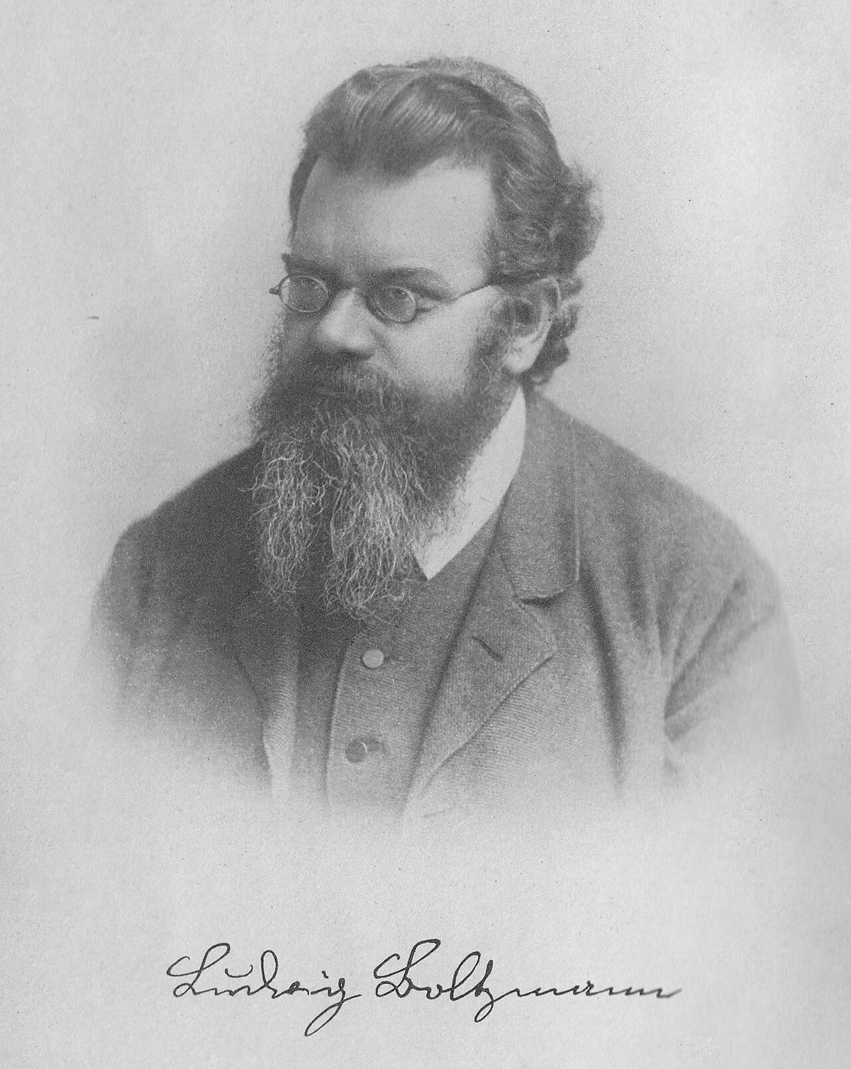
Ludwig Boltzmann (1844–1906), whose factor -E/k_BT is the subject of this chapter, and whose formula S = k_B is engraved on his tomb in Vienna. — Ludwig Boltzmann (1844–1906), whose factor $\eu^{-E/k_BT}$ is the subject of this chapter, and whose formula $S = k_B\ln\Omega$ is engraved on his tomb in Vienna.

29.7 Problem: The isothermal atmosphere, helium escape and a spin thermometer

Problem 29.1

Weekend problem — three uses of one exponential

Data: $k_B = 1.38 \times 10^{-23}\,\mathrm{J}/\mathrm{K}$ , $N_A = 6.02 \times 10^{23}\,\mathrm{mol}^{-1}$ , $g = 9.8\,\mathrm{m}/\mathrm{s}^{2}$ , $R_{\oplus} = 6.37 \times 10^{6}\,\mathrm{m}$ , $\mu_B = 9.27 \times 10^{-24}\,\mathrm{J}/\mathrm{T}$ ; air $M = 29\,\mathrm{g}/\mathrm{mol}$ , helium $4\,\mathrm{g}/\mathrm{mol}$ , nitrogen $28\,\mathrm{g}/\mathrm{mol}$ .

Part I — The isothermal atmosphere.

From hydrostatics and the perfect-gas law, derive $P(z) = P_0\eu^{-z/H}$ and give $H$ for air at $288\,\mathrm{K}$ .
Identify the Boltzmann factor in the result; which energy, which temperature?
Pressure at $3000\,\mathrm{m}$ , $5500\,\mathrm{m}$ and $8849\,\mathrm{m}$ ; the altitude where the pressure is halved.
Mass of the atmosphere per square metre (from $P_0 = 1.013 \times 10^{5}\,\mathrm{Pa}$ ), and the total mass; check that $\int_0^\infty \rho\,\dd z = \rho_0H$ .
Number of molecules in the atmosphere.
If each gas followed its own $H$ , what would be the ratio O $_2$ /N $_2$ at $50\,\mathrm{km}$ compared with the ground? Why is the composition in fact uniform up to $100\,\mathrm{km}$ ?
The real troposphere cools at $6.5\,\mathrm{K}/\mathrm{km}$ : is the pressure at $10\,\mathrm{km}$ higher or lower than the isothermal estimate? Explain.
Number density at sea level and at $100\,\mathrm{km}$ (isothermal model, $288\,\mathrm{K}$ ): comment on “the edge of space”.

Part II — Helium escape. The exosphere, above $500\,\mathrm{km}$ , is at about $1000\,\mathrm{K}$ and collisionless: a molecule moving upward faster than the escape speed leaves.

Escape speed from the Earth at that altitude.
Most probable and mean speeds of helium and nitrogen at $1000\,\mathrm{K}$ .
Fraction of helium atoms with $v > v_{\text{esc}}$ (use $(2/\sqrt\pi)x\eu^{-x^2}$ ); same for nitrogen.
The flux of escaping helium is roughly $\tfrac14n_{\text{He}}\langle v\rangle \times$ (that fraction) $\times\tfrac12$ ; with $n_{\text{He}} = 1 \times 10^{12}\,\mathrm{m}^{-3}$ at the exobase, estimate the loss per square metre per second and per year for the whole Earth.
Helium in the air is $5\,\mathrm{ppm}$ by volume: total helium in the atmosphere; its residence time against the loss computed.
Radioactivity in the crust produces about $3 \times 10^{6}\,\mathrm{kg}$ of helium per year: is the atmosphere’s helium in steady state, and what does the comparison with question 11 teach?
At solar maximum the exosphere reaches $2000\,\mathrm{K}$ : by what factor does the helium escape fraction rise?
Why does the Moon have no atmosphere, and Titan (escape $2.6\,\mathrm{km}/\mathrm{s}$ , $94\,\mathrm{K}$ ) a thick one?

Part III — A spin thermometer. A paramagnetic salt contains $n = 2 \times 10^{27}\,\mathrm{m}^{-3}$ spins 1/2 with $\mu = \mu_B$ , in a field $B$ .

Populations of the two levels and the magnetisation $M(B,T)$ .
At $B = 0.1\,\mathrm{T}$ : $M$ at $300\,\mathrm{K}$ , $4\,\mathrm{K}$ , $0.05\,\mathrm{K}$ ; where is Curie’s law valid?
Why is $M$ a thermometer, and in which range is it most sensitive? What is measured in practice?
Mean energy and heat capacity of the spins (Schottky); temperature of the peak at $0.1\,\mathrm{T}$ .
Entropy of the spins at high and at zero temperature; what “ordering” occurs as $T \to 0$ ?
Adiabatic demagnetisation from $1\,\mathrm{K}$ , $1\,\mathrm{T}$ to $0.01\,\mathrm{T}$ : final temperature; why cannot $B \to 0$ give $T \to 0$ ?
A nuclear-spin thermometer uses $\mu_{\text{N}} = \mu_B/1836$ : at $1\,\mathrm{T}$ , down to what temperature does Curie’s law hold, and why is such a thermometer used in the microkelvin range?
Compare the Doppler width of a spectral line (from Maxwell’s distribution) as a thermometer for gases: which quantity, and how does it scale with $T$ ?
Summarise: the three systems and the single formula.

Solution

Solution of Problem 29.1.

1. $\dd P/\dd z = -nmg = -(mg/k_BT)P$ ; $H = 8.4\,\mathrm{km}$ .

2. $\eu^{-mgz/k_BT}$ : the potential energy of one molecule, the air’s temperature.

3. $0.70\,$ , $0.52\,$ , $0.35\,\mathrm{bar}$ ; $H\ln 2 = 5.8\,\mathrm{km}$ .

4. $P_0/g = 1.03 \times 10^{4}\,\mathrm{kg}/\mathrm{m}^{2}$ ; $\times 4\pi R^2$ : $5.3 \times 10^{18}\,\mathrm{kg}$ ; $\rho_0H = 1.22 \times 8400 = 1.03 \times 10^{4}\,\mathrm{kg}/\mathrm{m}^{2}$ .

5. $5.3 \times 10^{18}/(29 \times 10^{-3}/N_A) = 1.1 \times 10^{44}$ .

6. $H_{\text{O}_2} = 7.6$ , $H_{\text{N}_2} = 8.7\,\mathrm{km}$ : the ratio at $50\,\mathrm{km}$ would be $\eu^{-50/7.6 + 50/8.7} = 0.44$ of its ground value; turbulence mixes faster than diffusion separates.

7. Lower: colder air is denser and the pressure falls faster.

8. $2.5 \times 10^{25}\,\mathrm{m}^{-3}$ ; $\eu^{-11.9}$ : $1.7 \times 10^{20}\,\mathrm{m}^{-3}$ — no edge, only a convention.

9. $11.2\sqrt{6370/6870} = 10.8\,\mathrm{km}/\mathrm{s}$ .

10. Helium $2040\,$ , $2300\,\mathrm{m}/\mathrm{s}$ ; nitrogen $770\,$ , $870\,\mathrm{m}/\mathrm{s}$ .

11. $x = 5.3$ : $4 \times 10^{-12}$ ; nitrogen $\eu^{-196}$ : none.

12. $\tfrac14 \times 10^{12} \times 2300 \times 4 \times 10^{-12} \times \tfrac12 \approx 10^3$ atoms per square metre per second; over the Earth and a year, $2 \times 10^{25}$ atoms — $0.1\,\mathrm{kg}$ .

13. $5 \times 10^{-6} \times 1.1 \times 10^{44} = 5.5 \times 10^{38}$ atoms, $3.7 \times 10^{12}\,\mathrm{kg}$ ; against $0.1\,\mathrm{kg}/\mathrm{yr}$ the residence time would be absurd.

14. Steady state requires a loss of $3 \times 10^{6}\,\mathrm{kg}/\mathrm{yr}$ : a residence time of about a million years, which is the accepted value — so the thermal estimate at $1000\,\mathrm{K}$ is far too small: the escape is dominated by hotter episodes and by non-thermal (ionic) processes.

15. $x = 3.75$ : $\eu^{-14}$ instead of $\eu^{-28}$ — a factor $10^6$ : the loss is extraordinarily sensitive to the exospheric temperature.

16. The Moon is hot and light: everything escapes in geological time; Titan is cold, $x = 11$ for nitrogen.

17. $p_\pm = \eu^{\pm x}/2\cosh x$ ; $M = n\mu\tanh x$ .

18. $x = \mu B/k_BT$ : $4.2\,\mathrm{A}/\mathrm{m}$ , $310\,\mathrm{A}/\mathrm{m}$ , $1.6 \times 10^{4}\,\mathrm{A}/\mathrm{m}$ (saturation $1.9 \times 10^{4}\,\mathrm{A}/\mathrm{m}$ ); Curie for $x \ll 1$ , i.e. $T \gg 70\,\mathrm{mK}$ .

19. $M$ depends on $T$ alone once $B$ is known; steepest near $x \approx 1$ , $T \approx \mu B/k_B = 70\,\mathrm{mK}$ ; one measures the susceptibility with a coil.

20. $\langle E\rangle = -N\mu B\tanh x$ ; $C = Nk_Bx^2/\cosh^2x$ , peaking at $x = 1.2$ : $56\,\mathrm{mK}$ .

21. $Nk_B\ln 2$ and $0$ : all the spins align with the field.

22. $10\,\mathrm{mK}$ ; the spins’ own field of a millitesla replaces $B$ and fixes the floor.

23. $x = 1$ at $\mu_{\text{N}}B/k_B = 0.37\,\mathrm{mK}$ : Curie holds down to a millikelvin, and the thermometer is useful to microkelvins.

24. $\Delta\nu/\nu = \sqrt{8k_BT\ln2/mc^2} \propto \sqrt T$ : the width of a line measures the gas temperature.

25. Atmosphere, escaping gas, spins: $\eu^{-E/k_BT}$ with $E = mgz$ , $\tfrac12mv^2$ , $\mp\mu B$ .