19The Phanerozoic Earth

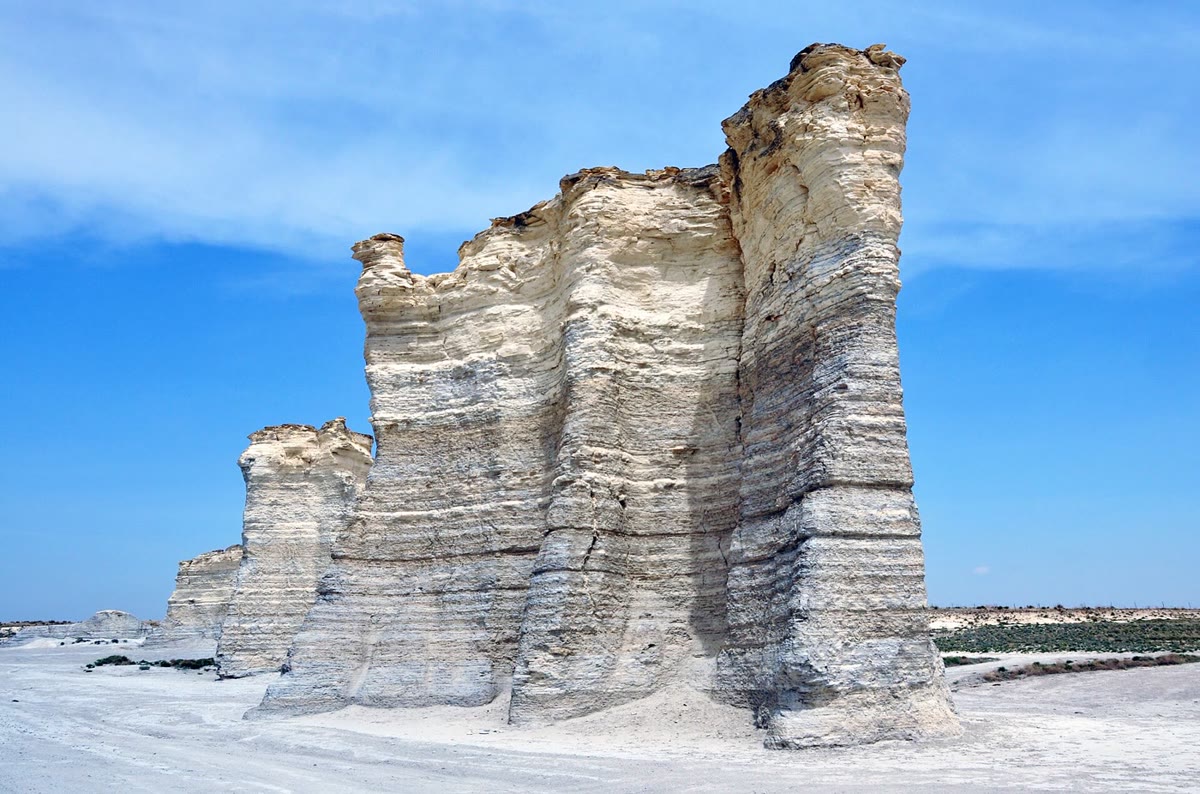
In western Kansas, in the middle of North America, pillars of white chalk rise from the prairie. The chalk is the ooze of a sea floor: about 80 million years ago a shallow sea ran from north to south across the middle of North America, and the shells of floating algae settled on its floor at a few hundredths of a millimetre a year. Five times in the last 540 million years, a large share of the species living in such seas vanished within a geological instant. Both stories are the Earth’s own: the continents moved and the sea rose and fell over them, and at least three of the five great extinctions fell on outpourings of lava from inside the planet. This chapter follows the Phanerozoic through its maps, its sea level, its mountain belts and its crises, and puts numbers on two of them: how fast ridges raise the sea, and how much land a higher sea drowns.

You already know

From the school volumes: plate tectonics and Pangaea; fossils and the geological time scale; transgressions read in a cliff. From the Year 1 volume: the depth–age law of the ocean floor; the hypsometric curve; isostasy; eustasy and relative sea level; large igneous provinces; mass extinctions as stratigraphic markers, the iridium of the K–Pg boundary and the dating of the end-Permian crisis; stages and GSSPs. From earlier chapters: orogens (Chapters 13 and 14); the Wilson cycle and supercontinents (Chapter 15); backstripping (Chapter 16); the snowballs of the Cryogenian (Chapter 18). Extinction and the history of life belong to the biology books; the Year 3 volume treats palaeomagnetism and sequence stratigraphy.

19.1 Maps of a moving world

A rock is rarely where it formed. A coal, a desert sandstone, a reef: each was laid down at some latitude and has been carried since by its plate. Before the climate or the life of a past time can be read from such rocks, they must be put back where they were.

Definition 19.1 (Palaeogeography; palaeogeographic map)

Palaeogeography is the reconstruction of the geography of a past time: the positions of the continents and oceans, and of their shorelines, mountain belts and seas. A palaeogeographic map shows that geography at one time, on the grid of latitude and longitude of that time.

Four kinds of evidence go into such a map. The magnetisation of rocks gives the latitude at which they formed, the subject of palaeomagnetism in the Year 3 volume; but the Earth’s field is symmetric about its axis, so it says nothing of longitude. The ocean floor records the motion of the plates directly, through its magnetic stripes and its ages, but only as far back as the oldest surviving floor, about 190 million years: anything older has been subducted. Before that, the fit of the continents, the sutures and orogens where oceans closed, and the fossils and sediments that betray a climate — reefs and evaporites in the tropics, glacial deposits near the poles — complete the picture. Plate models gather these constraints and turn every plate back in time; reconstructions also have to allow for the slow rotation of the whole solid Earth relative to its spin axis, called true polar wander.

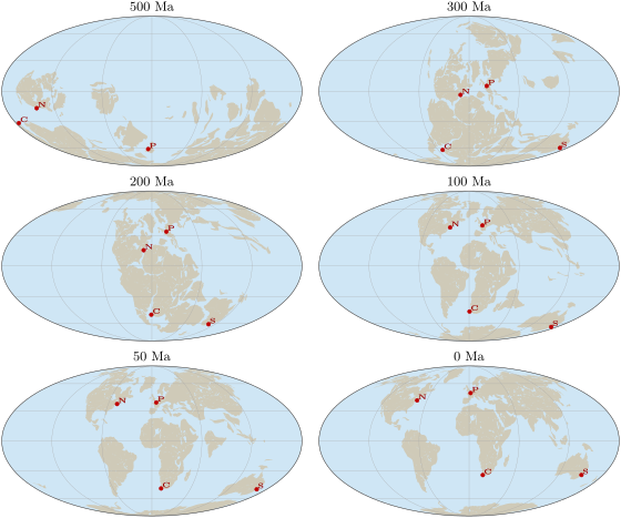
The six maps above are the Phanerozoic in brief. At $500\,\mathrm{Ma}$ the southern continents form one mass, Gondwana, much of it near the South Pole, with the crust of Paris at $61{}^{\circ}$ S on its margin. By $300\,\mathrm{Ma}$ the continents have joined into Pangaea, assembled from about $325\,\mathrm{Ma}$ and broken up from about $200\,\mathrm{Ma}$: Paris and New York lie on the equator, Cape Town and Sydney near $60{}^{\circ}$ S. At $200\,\mathrm{Ma}$ the supercontinent is complete, a single land stretching from high northern to high southern latitudes; by $100\,\mathrm{Ma}$ the Atlantic and the Indian Ocean have opened, and by $50\,\mathrm{Ma}$ the map is nearly today’s, with Australia still close to Antarctica.

Example 19.2 (Paris drifts north)

In the model, Paris lay at $5.1{}^{\circ}$ N $300\,\mathrm{Ma}$ ago; it lies today at $48.9{}^{\circ}$ N. Its latitude has grown by $43.8{}^{\circ}$, that is $43.8 \times 111.2 = 4871\,\mathrm{km}$ along a meridian ($111.2\,\mathrm{km}$ per degree on a sphere of radius $6371\,\mathrm{km}$), at a mean rate of $4871/300 = 16\,\mathrm{km}$ per million years, or $1.6\,\mathrm{cm}$ a year. This is only the northward part of the motion: the palaeomagnetic frame leaves the longitude free, so the true distance travelled was at least this.

19.2 Sea level through the Phanerozoic

Seas on the continents

Over most of the Phanerozoic, much more of the continents lay under the sea than today. The marine rocks of North America record several floods of the continent’s interior, the first of them the Cambrian transgression that seals the Great Unconformity; in the Late Cretaceous, from about 120 to $80\,\mathrm{Ma}$, marine sediments accumulated across the Western Interior, in the middle of the continent (photograph below).

Definition 19.3 (Epeiric sea)

An epeiric sea is a shallow sea spread over the interior of a continent, on continental crust, far from the continental margin.

The sea reaches such interiors by moving its shore, and the rocks record that motion.

Definition 19.4 (Marine transgression; marine regression)

A marine transgression is a landward shift of the shoreline, by which the sea spreads over the land; a marine regression is a seaward shift, by which the land emerges.

In a vertical section, a transgression stacks deeper-water deposits on shallower ones — offshore mud over beach sand — and a regression the reverse. Both follow the relative sea level, which mixes the global sea level with the subsidence or uplift of the place and with the supply of sediment: a delta can push its shore seaward while the sea rises, if it is fed fast enough. To read the global sea level from transgressions, a geologist must find the same signal on several continents, or remove the subsidence by backstripping, as in Chapter 16.

The long-term curve

Definition 19.5 (First-order sea-level cycle)

The first-order sea-level cycle is the slowest part of the change of global sea level, on time scales of tens to hundreds of millions of years, set by the tectonics of the solid Earth rather than by ice.

Across the Phanerozoic the first-order curve has the shape of an M: high in the early Palaeozoic, low while Pangaea assembled and stood, from the Carboniferous to the end of the Triassic, high again in the Cretaceous, and falling since. Extrapolated from North America, the flood of the Late Ordovician alone suggests a further rise of 100 to $200\,\mathrm{m}$. Faster changes ride on this curve: those driven by ice are recorded on time scales of $10^4$ to $10^6$ years, and the Antarctic ice sheet, from about $33.5\,\mathrm{Ma}$, moved the sea by 50 to $60\,\mathrm{m}$.

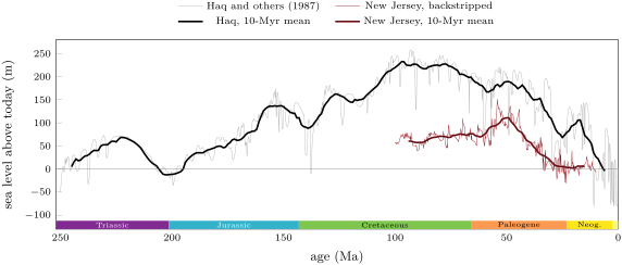
The two curves above agree on the shape and disagree on the size. The cycle chart, built from the stacking of sediments in many basins, puts the long-term sea level of the mid-Cretaceous about $233\,\mathrm{m}$ above today’s; the New Jersey wells, backstripped one by one, give about $70\,\mathrm{m}$ in the Late Cretaceous and a maximum near $110\,\mathrm{m}$ in the Eocene. Miller and his colleagues conclude that the long-term Cretaceous peak was $100 \pm 50\,\mathrm{m}$, and that the cycle charts, right about the timing of the falls, exaggerate their amplitudes. Even New Jersey is not a perfect gauge: its Late Cretaceous sea is 100 to $150\,\mathrm{m}$ lower than the volume of the ocean basins predicts, a gap that the sinking of the region above the subducted Farallon plate — dynamic topography — could explain.

Why the sea moves: ridges

What raises the sea by a hundred metres for tens of millions of years? Not ice: the Cretaceous was a warm world with at most small, short-lived ice sheets. The leading answer is the volume of the ocean ridges. Young ocean floor is hot and stands high; the faster the plates spread, the younger the floor is on average, the shallower the ocean basins, and the more water spills onto the continents.

Proposition 19.6 (Sea level and spreading rate)

Let ocean floor of area $A_{\text{f}}$ be made at ridges of total length $L$ at the full spreading rate $u$, and be destroyed at the age $\tau = A_{\text{f}}/(Lu)$, every age between 0 and $\tau$ covering the same area. Let its depth follow the law $d(t) = d_{\text{r}} + c\sqrt t$.

1. The mean depth of the floor is $\bar d = d_{\text{r}} + \tfrac23 c\sqrt\tau$.
2. If the spreading rate becomes $fu$, with $A_{\text{f}}$ and $L$ unchanged, the mean depth decreases by $\Delta\bar d = \tfrac23 c\sqrt\tau\,\bigl(1 - f^{-1/2}\bigr)$.

3. If the floor sinks isostatically under the added water, and the sea does not spread over the land, the sea level over an ocean of area $A_{\text{o}}$ rises by

   $$\Delta s = \frac{\rho_{\text{m}} - \rho_{\text{w}}}{\rho_{\text{m}}}\, \frac{A_{\text{f}}}{A_{\text{o}}}\,\Delta\bar d ,$$

   with $\rho_{\text{m}}$ the density of the mantle and $\rho_{\text{w}}$ that of sea water.

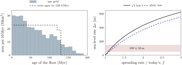
The real floor is not so tidy. Its ages are not evenly spread: young floor is the most abundant, and the area falls with age, as the left panel below shows. Nor does the square-root law hold for old floor, which flattens near $6.4\,\mathrm{km}$; the exponential law that Parsons and Sclater fitted to old floor, the plate law, takes over beyond about $26\,\mathrm{Myr}$, where the two laws meet. The proposition is a first estimate, and the figure shows how much the second law changes it.

Example 19.7 (Twice as fast)

Take the floor today: mean age $64.2\,\mathrm{Myr}$, so $\tau = 128.4\,\mathrm{Myr}$ in the even model; $d_{\text{r}} = 2500\,\mathrm{m}$, $c = 350\,\mathrm{m}\,\mathrm{Myr}^{-1/2}$. The mean depth is $2500 + \tfrac23 \times 350 \times \sqrt{128.4} = 5144\,\mathrm{m}$. Doubling the rate halves $\tau$, and the mean depth becomes $2500 + \tfrac23 \times 350 \times \sqrt{64.2} = 4370\,\mathrm{m}$: the floor rises by $774\,\mathrm{m}$ on average. With $A_{\text{f}}/A_{\text{o}} = 293/362 = 0.8094$ and $(\rho_{\text{m}} - \rho_{\text{w}})/\rho_{\text{m}} = (3300 - 1025)/3300 = 0.689$, the sea rises by $0.689 \times 0.8094 \times 774 = 432\,\mathrm{m}$; with the plate law, $368\,\mathrm{m}$. Both are about four times the long-term Cretaceous peak. Read the other way, the right panel says that a spreading rate only 15 to $20\,\%$ above today’s suffices for $100\,\mathrm{m}$ — which is why Miller and his colleagues conclude that ocean crust was made much more slowly in the Cretaceous than once inferred.

The model is also too deep: its mean depth, $5144\,\mathrm{m}$, exceeds the measured mean depth of the dated floor, $4265\,\mathrm{m}$, partly because the square-root law overshoots on old floor, and partly because the real floor carries sediment, seamounts and plateaus that the law leaves out. And spreading is not the only lever. Ridges are balanced by trenches: if the ocean floor rises in one place, the mass must go somewhere, and a continent sinking over a slab — dynamic topography — lets the sea in locally. Tasistro-Hart and Macdonald argue that the floods of North America follow the slabs under the continent, and that the global sea level depends on how much subduction happens under continents rather than under oceans.

19.3 Flooding the continents

How much land a rise of the sea drowns depends on the shape of the Earth’s surface, which the hypsometric curve of the Year 1 volume summarises: the fraction of the surface that stands above each elevation (figure below, left). The continents are flat-topped. On the one-degree grid of ETOPO1, $29.0\,\%$ of the surface is land and $34.3\,\%$ stands above $-200\,\mathrm{m}$: the shelves, already under water, make the difference. Most land is low, so a modest rise floods a great deal of it.

Proposition 19.8 (Flooding the land)

Let $A_{\text{o}}$ be the area of the sea today and $a(z)$ the area of land lower than $z$ above today’s sea level. A volume $V$ of water added to the sea raises its level by the height $s$ that solves

$$V = \int_0^s \bigl(A_{\text{o}} + a(z)\bigr)\,\mathrm{d}z ,$$

and floods the land area $a(s)$. Since $a \ge 0$, the rise is at most $V/A_{\text{o}}$.

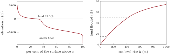
The right panel gives the answer at once. A rise of $100\,\mathrm{m}$ drowns about $15\,\%$ of today’s land; the $432\,\mathrm{m}$ of a doubled spreading rate would drown half. Such a sea spreads over the land it floods, so the rise itself is smaller than the proposition’s bound $V/A_{\text{o}}$, by about a tenth for a rise of a few hundred metres (weekend problem). The Cretaceous seas of Kansas needed far less: the interior of a continent is often low, and it may also sink over a slab.

19.4 Mountain belts of the Phanerozoic

Each Wilson cycle of Chapter 15 ends in a mountain belt, and the Phanerozoic belts mark the making and the breaking of Pangaea. The table gathers those met in this volume.

The first two belts sewed Pangaea together, the Variscan closing the last ocean between Gondwana and Laurussia; the last three grew as the pieces of Pangaea moved apart and the oceans between them were consumed. The low sea level of the late Palaeozoic and Triassic belongs to this supercontinent, and the high sea of the Cretaceous to its break-up, with new ridges and young floor.

19.5 Crises of life

The big five

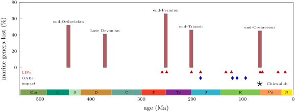
The biology volumes describe mass extinctions; geologists measure them in the rocks and look for their causes. Five stand out in the record of marine animals, the “big five”: at the end of the Ordovician, about $444\,\mathrm{Ma}$; in the Late Devonian, $372\,\mathrm{Ma}$; at the end of the Permian, $251.9\,\mathrm{Ma}$; at the end of the Triassic, $201.4\,\mathrm{Ma}$; and at the end of the Cretaceous, $66\,\mathrm{Ma}$. Each removed between about two fifths and two thirds of the genera of marine animals in Sepkoski’s compilation. The end-Permian crisis was the largest: $56\,\%$ of genera at the finest resolution, and about $81\,\%$ of marine species — not the $96\,\%$ often quoted, which mixed two separate crises.

History — The big five, forty years on

In 1982, D. M. Raup and J. J. Sepkoski counted the families of marine animals that disappeared in each of 76 stages of the Phanerozoic. Four points stood above the 99 per cent confidence limit of their trend — the last stage of the Ordovician, the last two of the Permian and the last of the Cretaceous — and the end of the Triassic and the end of the Devonian above the 95 per cent limit: the big five. Forty years later, the five remain the largest crises since the early Ordovician, but with better data they no longer stand apart from a continuum of extinction rates, and some intervals of the Cambrian had even higher rates. Raup and Sepkoski’s time resolution was $7.4\,\mathrm{Myr}$, the mean length of a stage then; some crises were sudden, others lasted hundreds of thousands of years or longer.

Large igneous provinces

The figure above shows the pattern that the Year 1 volume pointed to: the three most recent of the big five each fall on a large igneous province, the Siberian Traps at the end of the Permian, the Central Atlantic Magmatic Province (CAMP) at the end of the Triassic, the Deccan Traps at the end of the Cretaceous. The proposed link is the gas. A flood basalt erupts in pulses of a few centuries to a few millennia, each releasing carbon dioxide faster than weathering can take it back; the sulfur of the same eruptions cools the climate briefly, the carbon warms it for much longer and acidifies the ocean.

Example 19.9 (The carbon of the Central Atlantic province)

Gas bubbles in melt inclusions of CAMP basalts show that the magma held at least 0.5 to $0.6\,\%$ of carbon dioxide by mass. Take $0.55\,\%$, a density of $2900\,\mathrm{kg}\,\mathrm{m}^{-3}$ and a volume of $5.5 \times 10^{6}\,\mathrm{km}^{3}$, the erupted lavas with the dykes, sills and chambers that fed them. The mass of magma is $5.5 \times 10^{6} \times 10^{9} \times 2900 = 1.6 \times 10^{19}\,\mathrm{kg}$, and its carbon dioxide $1.6 \times 10^{19} \times 0.0055 = 8.8 \times 10^{16}\,\mathrm{kg}$, about $9 \times 10^{4}\,\mathrm{Gt}$ — the authors’ “up to $10^{5}\,\mathrm{Gt}$”. Released over the province’s lifetime, it was not all in the air at once; but each pulse, of the order of $10^{5}\,\mathrm{km}^{3}$ in a few centuries, released as much as the emissions projected for the twenty-first century.

Oceanic anoxic events

Not every crisis is one of the big five. Several times in the Mesozoic, oxygen disappeared from large parts of the ocean.

Definition 19.10 (Oceanic anoxic event)

An oceanic anoxic event (OAE) is an interval of widespread oxygen depletion in the ocean, recognised in the sedimentary and geochemical record.

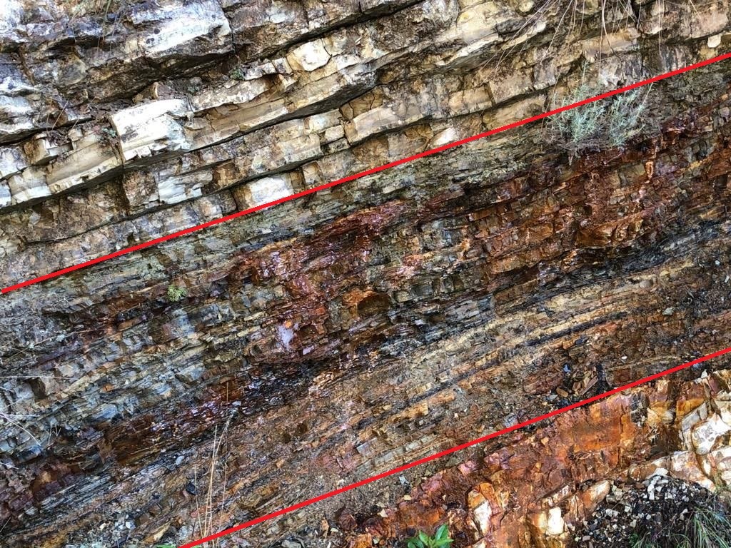
Its usual mark is a black shale: dark, finely laminated, without burrows, rich in organic matter and in pyrite, often with a shift of the carbon isotopes and signs of warming. The best studied are the early Toarcian event, about $183\,\mathrm{Ma}$, the early Aptian OAE 1a, about $120\,\mathrm{Ma}$, the early Albian OAE 1b, about $111\,\mathrm{Ma}$, and OAE 2 at the boundary between the Cenomanian and the Turonian, about $94\,\mathrm{Ma}$, in the hottest part of the Cretaceous, when the sea stood exceptionally high. Several coincide with a province: the Toarcian event with the Karoo–Ferrar basalts, OAE 1a with the Ontong Java Plateau. OAE 2 is often tied to the Caribbean plateau, but mercury spikes in Southern Hemisphere sediments point to the Kerguelen province instead.

In the field — Logging an anoxic event

A geologist who studies an OAE in a section of pelagic limestones logs it bed by bed: thickness, colour, lamination, burrows or their absence, nodules of pyrite. She samples at close, regular intervals across the dark interval and well beyond it, for the organic carbon content and for the carbon isotopes of the organic matter and of the carbonate; the shift of the isotopes, more than the colour of the rock, correlates the event from one basin to the next. Because the darkest shale can appear at different levels in different basins, the isotope curve, not the black shale, is taken as the time line.

Chicxulub

The end of the Cretaceous had a cause from outside. The Year 1 volume told how the iridium of the boundary clay led to an impact, and how argon dating tied the boundary to the Chicxulub crater. The structure is about $200\,\mathrm{km}$ across and $66\,\mathrm{Ma}$ old; its hot rocks fed circulating water for at least eight million years after. Models of its subsurface asymmetry point to an impactor that came from the north-east at 45 to $60{}^{\circ}$ to the horizontal, at no less than the Earth’s escape velocity, $11.2\,\mathrm{km}\,\mathrm{s}^{-1}$, and more probably about $20\,\mathrm{km}\,\mathrm{s}^{-1}$. The Deccan Traps were erupting at the same time, before and after the impact; a review of the evidence in 2010 concluded that the impact triggered the extinction.

Figures as of 2026

The ages in this chapter are those of the International Chronostratigraphic Chart in its June 2026 version, as used throughout this series; the sea-level records are on the 2012 time scale of their files, and the extinction ages are those of Kaiho (2022). The chart is revised as new dates come in: check the current version before quoting a boundary age.

Exercises

Data for the exercises, unless stated otherwise: $111.2\,\mathrm{km}$ per degree of latitude; depth of the ocean floor $d(t) = 2500 + 350\sqrt t$ ($\mathrm{m}$, $t$ in $\mathrm{Myr}$); ocean area $362\,\mathrm{M}\mathrm{km}^{2}$; ocean floor area $293\,\mathrm{M}\mathrm{km}^{2}$; mantle density $3300\,\mathrm{kg}\,\mathrm{m}^{-3}$; sea water $1025\,\mathrm{kg}\,\mathrm{m}^{-3}$; mass of the atmosphere $5.1 \times 10^{18}\,\mathrm{kg}$, molar masses of air and of carbon dioxide $28.97\,\mathrm{g}\,\mathrm{mol}^{-1}$ and $44.01\,\mathrm{g}\,\mathrm{mol}^{-1}$.

Exercise 19.1 ★

In the model of the maps, Cape Town lay at $61.9{}^{\circ}$ S $300\,\mathrm{Ma}$ ago and New York at $3.6{}^{\circ}$ S; today they lie at $33.9{}^{\circ}$ S and $40.7{}^{\circ}$ N. (a) Which of the four cities lay within $30{}^{\circ}$ of the equator $300\,\mathrm{Ma}$ ago (Paris at $5.1{}^{\circ}$ N, Sydney at $59.5{}^{\circ}$ S)? (b) How far north, in kilometres, has each of Cape Town and New York moved since? (c) At what mean rates, in centimetres a year?

Solution

Solution of Exercise 19.1.

(a) Paris ($5.1{}^{\circ}$ N) and New York ($3.6{}^{\circ}$ S); Cape Town and Sydney lay near $60{}^{\circ}$ S. (b) Cape Town: $61.9 - 33.9 = 28.0{}^{\circ}$, $28.0 \times 111.2 = 3114\,\mathrm{km}$; New York: $40.7 + 3.6 = 44.3{}^{\circ}$, $4926\,\mathrm{km}$. (c) $3114/300 = 10.4\,\mathrm{km}$ per million years, $1.0\,\mathrm{cm}$ a year; $4926/300 = 16.4\,\mathrm{km}$ per million years, $1.6\,\mathrm{cm}$ a year.

Exercise 19.2 ★

The big five fell at 444, 372, 251.9, 201.4 and $66\,\mathrm{Ma}$. (a) Find the intervals between successive crises and their mean. (b) Using the mean ages of the large igneous provinces — Emeishan 259, Siberian 250, CAMP 201, Karoo–Ferrar 183, Deccan $65.5\,\mathrm{Ma}$ — which of the five fall within $2\,\mathrm{Myr}$ of a province? (c) Does a mean interval make the crises periodic?

Solution

Solution of Exercise 19.2.

(a) 72, 120.1, 50.5 and $135.4\,\mathrm{Myr}$; mean $(444 - 66)/4 = 94.5\,\mathrm{Myr}$. (b) The end-Permian (Siberian, $1.9\,\mathrm{Myr}$ apart), the end-Triassic (CAMP, $0.4\,\mathrm{Myr}$) and the end-Cretaceous (Deccan, $0.5\,\mathrm{Myr}$). (c) No: the intervals range from 50 to $135\,\mathrm{Myr}$; a mean exists for any set of dates.

Exercise 19.3 ★

The chalk of Monument Rocks was laid down at about $0.036\,\mathrm{mm}$ a year. (a) How long did $91\,\mathrm{m}$ of it take? (b) How many times faster does the sea rise today, at $3.7\,\mathrm{mm}$ a year? (c) Why can a sea floor collect such a slow rain of sediment without being buried by mud?

Solution

Solution of Exercise 19.3.

(a) $91\,\mathrm{m}/0.036\,\mathrm{mm}\,\mathrm{yr}^{-1} = 2.5 \times 10^{6}$ years. (b) $3.7/0.036 = 103$ times. (c) Far from any shore, in clear water, little mud from rivers reached the floor; the rain of algal shells was the main sediment.

Exercise 19.4 ★

In a cliff, from the bottom up: river sandstone with roots, beach sand with shells, grey offshore mud, chalk; then the chalk is overlain by beach sand again. (a) Where does the section record a marine transgression, and where a regression? (b) Does the transgression prove that global sea level rose? (c) What would make it more convincing?

Solution

Solution of Exercise 19.4.

(a) From the river sandstone to the chalk the deposits deepen upwards: a transgression. The beach sand above the chalk records a regression. (b) No: it records a rise of relative sea level, which subsidence of the place, or a drop in the supply of sediment, could also produce. (c) Finding the same transgression, at the same time, on other continents, or removing the subsidence by backstripping.

Exercise 19.5 ★★

On the long-term curve of Haq and others, sea level stood $233\,\mathrm{m}$ above today’s at $97\,\mathrm{Ma}$. (a) What mean rate of fall since then, in metres per million years and in micrometres a year? (b) Compare with today’s rise of $3.7\,\mathrm{mm}$ a year. (c) The backstripped New Jersey curve gives about $70\,\mathrm{m}$ at the same time. Which would you trust for the amplitude, and why?

Solution

Solution of Exercise 19.5.

(a) $233/97 = 2.4\,\mathrm{m}$ per million years, $2.4\,\text{µ}\mathrm{m}$ a year. (b) $3.7/0.0024 = 1540$: today’s rise is some 1500 times faster. (c) The backstripped curve: drilling has shown that cycle charts get the timing of falls right but overstate their size, by a factor of two or more; New Jersey has its own bias (dynamic topography), hence the estimate of $100 \pm 50\,\mathrm{m}$.

Exercise 19.6 ★★

A single pulse of the CAMP, about $10^{5}\,\mathrm{km}^{3}$ of basalt of density $2900\,\mathrm{kg}\,\mathrm{m}^{-3}$, erupted in about 500 years. (a) With $0.75\,\%$ of carbon dioxide by mass, how much did it release, in kilograms and in moles? (b) What mass of carbon dioxide did the air hold at the $278\,\mathrm{ppm}$ of 1750? (c) Compare. (d) How many such atmospheres would the whole province, $10^{5}\,\mathrm{Gt}$, have provided?

Solution

Solution of Exercise 19.6.

(a) $10^{5} \times 10^{9} \times 2900 = 2.9 \times 10^{17}\,\mathrm{kg}$ of basalt, and $2.9 \times 10^{17} \times 0.0075 = 2.2 \times 10^{15}\,\mathrm{kg}$ of carbon dioxide, $2.2 \times 10^{15}/0.04401 = 4.9 \times 10^{16}\,\mathrm{mol}$. (b) $278 \times 10^{-6} \times (44.01/28.97) \times 5.1 \times 10^{18} = 2.15 \times 10^{15}\,\mathrm{kg}$. (c) One pulse released about as much as the whole air held in 1750. (d) $10^{17}/2.15 \times 10^{15} = 46.5$: nearly fifty.

Exercise 19.7 ★★

Take the Chicxulub impactor as a sphere $10\,\mathrm{km}$ across, of density $2630\,\mathrm{kg}\,\mathrm{m}^{-3}$. (a) Find its mass. (b) Find its kinetic energy at the least possible speed, $11.2\,\mathrm{km}\,\mathrm{s}^{-1}$, and at $20\,\mathrm{km}\,\mathrm{s}^{-1}$. (c) The Earth loses $47\,\mathrm{TW}$ of internal heat through its surface. How many years of that loss does each energy represent?

Solution

Solution of Exercise 19.7.

(a) $2630 \times \frac{\pi}{6} \times (10^{4})^3 = 1.38 \times 10^{15}\,\mathrm{kg}$. (b) $\tfrac12 \times 1.38 \times 10^{15} \times (11.2 \times 10^{3})^2 = 8.7 \times 10^{22}\,\mathrm{J}$; at $20\,\mathrm{km}\,\mathrm{s}^{-1}$, $2.76 \times 10^{23}\,\mathrm{J}$. (c) A year of $47\,\mathrm{TW}$ is $47 \times 10^{12} \times 3.156 \times 10^{7} = 1.48 \times 10^{21}\,\mathrm{J}$: 59 and 186 years.

Exercise 19.8 ★★

(a) List the features by which a black shale records an oceanic anoxic event. (b) Pair each event with a province of nearly the same age: early Toarcian, $183\,\mathrm{Ma}$; OAE 1a, $120\,\mathrm{Ma}$; given Karoo–Ferrar at $183\,\mathrm{Ma}$ and Ontong Java at $122\,\mathrm{Ma}$. (c) Why is a coincidence of ages not enough to prove that a province caused an event?

Solution

Solution of Exercise 19.8.

(a) Dark colour, fine lamination, no burrows, much organic matter, pyrite; often a shift of the carbon isotopes and signs of warming. (b) The Toarcian event with the Karoo–Ferrar, OAE 1a with Ontong Java. (c) Dates carry uncertainties of up to millions of years, and many events and provinces exist, so chance coincidences are likely; a causal link needs the province to start just before the event and a tracer of the volcanism, such as mercury, in the same sediments.

Exercise 19.9 ★★

In the model, Paris lay at $60.9{}^{\circ}$ S $500\,\mathrm{Ma}$ ago and at $5.1{}^{\circ}$ N $300\,\mathrm{Ma}$ ago. (a) Find its northward displacement in degrees and in kilometres, and the mean rate in centimetres a year. (b) Compare with the rate since $300\,\mathrm{Ma}$ (Example 19.2). (c) Why is the rate a minimum?

Solution

Solution of Exercise 19.9.

(a) $60.9 + 5.1 = 66.0{}^{\circ}$, $66.0 \times 111.2 = 7339\,\mathrm{km}$ in $200\,\mathrm{Myr}$: $36.7\,\mathrm{km}$ per million years, $3.7\,\mathrm{cm}$ a year. (b) More than twice the $1.6\,\mathrm{cm}$ a year since $300\,\mathrm{Ma}$. (c) Only the change of latitude is known; the change of longitude, free in a palaeomagnetic frame, and any detour add to the distance.

Exercise 19.10 ★★★

Suppose instead that the area of floor falls linearly with age, from a maximum at age 0 to zero at age $T$. (a) Show that the mean age is $T/3$ and that the mean of $\sqrt t$ is $\tfrac{8}{15}\sqrt T$. (b) With a mean age of $64.2\,\mathrm{Myr}$, find $T$ and the mean depth. (c) Find the fall of the mean depth when the spreading rate doubles, and compare with the $774\,\mathrm{m}$ of the even model. (d) Show that in both models the fall is close to $0.93\,c\sqrt{\bar t}\,(1 - f^{-1/2})$, with $\bar t$ the mean age.

Solution

Solution of Exercise 19.10.

(a) The fraction of floor of age $t$ is $p(t) = \frac2T(1 - t/T)$. Then $\int_0^T tp\,\mathrm{d}t = \frac2T\bigl(\frac{T^2}2 - \frac{T^2}3\bigr) = \frac T3$ and $\int_0^T \sqrt t\,p\,\mathrm{d}t = \frac2T\bigl(\frac23 T^{3/2} - \frac25 T^{3/2}\bigr) = \frac8{15}\sqrt T$. (b) $T = 3 \times 64.2 = 192.6\,\mathrm{Myr}$; $2500 + \frac8{15} \times 350 \times 13.878 = 5091\,\mathrm{m}$. (c) $T/2 = 96.3\,\mathrm{Myr}$: $4332\,\mathrm{m}$; the fall is $759\,\mathrm{m}$, $2\,\%$ less than $774\,\mathrm{m}$. (d) Even model: $\frac23\sqrt\tau = \frac23\sqrt{2\bar t} = 0.943\sqrt{\bar t}$; triangle: $\frac8{15}\sqrt{3\bar t} = 0.924\sqrt{\bar t}$. The answer depends on the mean age far more than on the shape.

Exercise 19.11 ★★★

(a) From Proposition 19.6, show that $\Delta s(f) = \Delta s(2)\,(1 - f^{-1/2})/(1 - 2^{-1/2})$. (b) With $\Delta s(2) = 432\,\mathrm{m}$, find the range of $f$ that gives the Cretaceous peak, 50 to $150\,\mathrm{m}$. (c) What would a spreading rate slowed to 0.8 of today’s do? (d) Why is a long-term sea level set by ridges a slow signal, whatever the change of rate?

Solution

Solution of Exercise 19.11.

(a) In $\Delta s$, only the factor $1 - f^{-1/2}$ depends on $f$; divide by its value at $f = 2$, $1 - 2^{-1/2} = 0.2929$. (b) $f = (1 - 0.2929\,\Delta s/432)^{-2}$: 1.071 for $50\,\mathrm{m}$, 1.239 for $150\,\mathrm{m}$; 7 to $24\,\%$ faster than today. (c) $432 \times (1 - 0.8^{-1/2})/0.2929 = -174\,\mathrm{m}$: the sea would fall by $174\,\mathrm{m}$. (d) The age spread changes only as old floor is subducted and replaced, which takes a time of the order of $\tau$, about $100\,\mathrm{Myr}$; the sea follows over tens of millions of years.

Exercise 19.12 ★★★

Suppose species die out at a constant rate, so that the fraction of a cohort that survives a time $t$ is $2^{-t/m}$, with a median species longevity $m = 2\,\mathrm{Myr}$. (a) What fraction of a cohort is gone after $7.4\,\mathrm{Myr}$, the mean stage length of the 1982 analysis? (b) How long would background extinction take to remove $81\,\%$ of species? (c) The end-Permian crisis lasted about $60\,\mathrm{kyr}$. How much faster was it? (d) Why does a coarse time resolution blur the difference between a mass extinction and a background one?

Solution

Solution of Exercise 19.12.

(a) $2^{-7.4/2} = 0.077$: $92\,\%$ gone. (b) $t = 2\log_2(1/0.19) = 4.8\,\mathrm{Myr}$. (c) $4.8/0.060 = 80$ times faster. (d) Within a long stage, background extinction alone removes most species, so a short pulse adds to a large total and is hard to separate from it; the incompleteness of the record also smears last appearances backwards.

Problem 19.1

Weekend problem — When the ridges were fast

This problem asks how much the sea would rise, and how much land it would drown, if the ridges spread twice as fast. Use the data of the exercises; the mean age of the ocean floor is $64.2\,\mathrm{Myr}$, the ridges are $65\,000\,\mathrm{km}$ long in all, today’s ocean holds $1.33 \times 10^{9}\,\mathrm{km}^{3}$, and the land covers $148\,\mathrm{M}\mathrm{km}^{2}$. The table gives the per cent of today’s land lying less than $h$ above sea level, from the one-degree ETOPO1 grid.

$h$ ($\mathrm{m}$)	0	100	200	300	400	500
land below $h$ ($\%$)	0	14.9	28.2	38.7	48.1	55.8

Assume, as in Proposition 19.6, that every age of floor between 0 and the age $\tau$ at which it is subducted covers the same area.

Part I — The ocean floor today.

1. Find the depth of the floor at ages 0, 25, 64.2 and $100\,\mathrm{Myr}$.
2. Find $\tau$ from the mean age, and the depth of the oldest floor.
3. Find the mean full spreading rate $u = A_{\text{f}}/(L\tau)$, in kilometres per million years and in millimetres a year. Is it a slow, intermediate or fast rate?
4. Show that the mean depth of the floor is $2500 + \tfrac23 \times 350\sqrt\tau$, and compute it.
5. The measured mean depth of the dated floor is $4265\,\mathrm{m}$. Give two reasons why the model is deeper.
6. What volume of water would lie above the floor in the model? Compare with the volume of the whole ocean.

Part II — A ridge in cross-section.

7. Find the half spreading rate $v$, to the nearest $0.1\,\mathrm{km}\,\mathrm{Myr}^{-1}$, and the width of floor on each side of the ridge.
8. How deep is the floor $1000\,\mathrm{km}$ from the axis?
9. Show that the cross-section of the ridge above the depth of the oldest floor, counting both flanks, has the area $\tfrac23 v c\,\tau^{3/2}$, and compute it in square kilometres.
10. Find the volume of the whole ridge system above that depth.
11. What fraction of the volume of the ocean is that?
12. Why does a ridge spreading faster stand higher on average?

Part III — Twice as fast.

13. The spreading rate doubles with the same floor area and ridge length. Find the new $\tau$ and the new mean depth.
14. By how much does the mean depth fall?
15. What volume of water does the floor push out of the basins?
16. Spread over today’s ocean, how much would it raise the sea?
17. Include the sinking of the floor under the extra water to find the rise $\Delta s$.
18. The long-term Cretaceous peak was about $100\,\mathrm{m}$. What increase of the spreading rate would give that?

Part IV — The sea over the land.

19. What area of land would a rise of $100\,\mathrm{m}$ flood?
20. What area would a rise of $432\,\mathrm{m}$ flood, by interpolation in the table?
21. Why must the sea rise by less than $432\,\mathrm{m}$ once it spreads over the land?
22. Find the volume needed to raise the sea in steps of $100\,\mathrm{m}$ up to $400\,\mathrm{m}$, averaging the flooded area over each step (Proposition 19.8). The volume to place is $0.432\,\mathrm{km} \times 362\,\mathrm{M}\mathrm{km}^{2}$. Where does the sea stop?
23. What per cent of today’s land does it then cover?
24. To sum up: in this model, by how much would doubling the spreading rate raise the sea?

Solution

Solution of Problem 19.1.

1. 2500, 4250, 5304 and $6000\,\mathrm{m}$. 2. $\tau = 2 \times 64.2 = 128.4\,\mathrm{Myr}$; $2500 + 350\sqrt{128.4} = 6466\,\mathrm{m}$. 3. $293 \times 10^{6}/(65000 \times 128.4) = 35.1\,\mathrm{km}$ per million years, $35.1\,\mathrm{mm}$ a year: a slow rate. 4. $\frac1\tau\int_0^\tau(2500 + 350\sqrt t)\,\mathrm{d}t = 2500 + \frac23 \times 350\sqrt\tau = 5144\,\mathrm{m}$. 5. The square-root law is too deep for floor older than a few tens of millions of years, which flattens; the real ages are not evenly spread, young floor being the most abundant; and sediment, seamounts and plateaus raise the floor. 6. $293 \times 10^{6} \times 5.144 = 1.51 \times 10^{9}\,\mathrm{km}^{3}$, $13\,\%$ more than the whole ocean: the model is too deep. 7. $v = 17.6\,\mathrm{km}$ per million years; $17.6 \times 128.4 = 2260\,\mathrm{km}$ on each side. 8. $t = 1000/17.6 = 56.8\,\mathrm{Myr}$; $2500 + 350\sqrt{56.8} = 5138\,\mathrm{m}$. 9. On one flank, with $x = vt$: $\int_0^{v\tau}\bigl(d(\tau) - d(x/v)\bigr)\mathrm{d}x = vc\int_0^\tau(\sqrt\tau - \sqrt t)\,\mathrm{d}t = \frac13 vc\,\tau^{3/2}$; twice that for both. $\frac23 \times 17.6 \times 0.350 \times 128.4^{3/2} = \frac23 \times 17.6 \times 0.350 \times 1454.9 = 5975\,\mathrm{km}^{2}$. 10. $65000 \times 5975 = 3.88 \times 10^{8}\,\mathrm{km}^{3}$. 11. $3.88 \times 10^{8}/1.33 \times 10^{9} = 0.29$. 12. Its floor is younger on average, so hotter, less dense and higher; the band of young floor along the axis is wider. 13. $\tau = 64.2\,\mathrm{Myr}$; $2500 + \frac23 \times 350\sqrt{64.2} = 4370\,\mathrm{m}$. 14. $5144 - 4370 = 774\,\mathrm{m}$. 15. $293 \times 10^{6} \times 0.774 = 2.27 \times 10^{8}\,\mathrm{km}^{3}$. 16. $2.27 \times 10^{8}/362 \times 10^{6} = 0.627\,\mathrm{km}$, $627\,\mathrm{m}$. 17. $\Delta s = 627 \times (3300 - 1025)/3300 = 432\,\mathrm{m}$. 18. $f = \bigl(1 - 0.2929 \times 100/432\bigr)^{-2} = 1.15$: $15\,\%$ faster. 19. $0.149 \times 148 = 22.1\,\mathrm{M}\mathrm{km}^{2}$. 20. $48.1 + 0.32 \times 7.7 = 50.6\,\%$, $74.9\,\mathrm{M}\mathrm{km}^{2}$. 21. As it rises it covers more area, so the same volume makes a thinner layer (Proposition 19.8). 22. Flooded areas at 100, 200, 300 and $400\,\mathrm{m}$: 22.1, 41.7, 57.3 and $71.2\,\mathrm{M}\mathrm{km}^{2}$. Steps: $(362 + 11.0) \times 0.1 = 37.3 \times 10^{6}\,\mathrm{km}^{3}$, then 39.4, 41.2 and $42.6 \times 10^{6}\,\mathrm{km}^{3}$; cumulated 37.3, 76.7, 117.9 and $160.5 \times 10^{6}\,\mathrm{km}^{3}$. The volume to place is $156.4 \times 10^{6}\,\mathrm{km}^{3}$, between 300 and $400\,\mathrm{m}$: $300 + (156.4 - 117.9)/42.6 \times 100 = 390\,\mathrm{m}$. 23. $38.7 + 0.90 \times 9.4 = 47.2\,\%$ of today’s land. 24. Doubling the spreading rate would raise the sea by about $390\,\mathrm{m}$ and drown nearly half of today’s land.