বইগুলো এখনো বাংলা ভাষায় পাওয়া যায় না — ইংরেজি সংস্করণ দেখানো হচ্ছে।
University Earth and Space Sciences — Year 2 · স্নাতক দ্বিতীয় বর্ষ
13Anatomy of a Mountain Belt: The Alps
The summit of the Matterhorn is made of gneiss and gabbro that once belonged to the margin of Apulia, the continent that lay on Africa’s side of a vanished ocean. The slopes below it are that ocean’s floor, serpentinite, gabbro and pillow basalt turned to eclogite, and beneath that, in the neighbouring Monte Rosa, lies the edge of Europe. Climbing through the pile, one crosses from one continent, through an ocean, to the other. This chapter reads the Alps as such a pile: where its pieces came from, how they were stacked, how much ground the stacking ate, and what the geophysics sees underneath.
You already know
From the high-school volume: continental collision, the suture, the shortening of a layer (the fraction of its length lost), reverse faults and thrusts. From the Year 1 volume: geological maps and cross-sections; normal, reverse and thrust faults, folds and vergence; passive margins; the oceanic crust, pillow lava and the sheeted dyke complex; active margins and the accretionary prism; isostasy, Airy’s root and the Bouguer anomaly; the foreland basin named among sedimentary basins. From Chapter 10: the blueschist and eclogite facies. From Chapter 11: P–T–t paths, exhumation rates and ultrahigh-pressure metamorphism.
Definition 13.1 (Orogen)
An orogen is a belt of the lithosphere shortened and thickened by the convergence of two plates, together with the rocks deformed and metamorphosed in it; the mountain range is its surface expression, the thickened crust beneath is its root.
13.1 A vanished ocean
The Alps record the closure of oceans while the African and European plates converged. The main one is the Alpine Tethys, made of two branches. Its southern branch, the Piemont–Liguria ocean, began to drift apart in the Middle Jurassic, as the Central Atlantic opened: the Alpine Tethys belongs kinematically to the opening of the Atlantic, unlike the Tethyan oceans further east. Radiolarites, siliceous oozes of the deep sea turned to rock, and aptychus limestones followed the onset of spreading, and they still identify its remnants. A narrow northern branch, the Valais ocean, probably opened in the earliest Cretaceous. Between the two lay a sliver of continent, the Briançonnais ribbon, which thins out eastwards and is absent from the eastern Alps.
To the north the ocean was bordered by Europe’s passive margin, the subject of the rift and margin chapter of the Year 1 volume. To the south lay Apulia: all the continental ground south of the Alpine Tethys and north of the younger Neotethys, including the foreland that now lies south of the Alps. The Matterhorn’s summit is a piece of it.
The map below locates the belt and the places of this chapter.
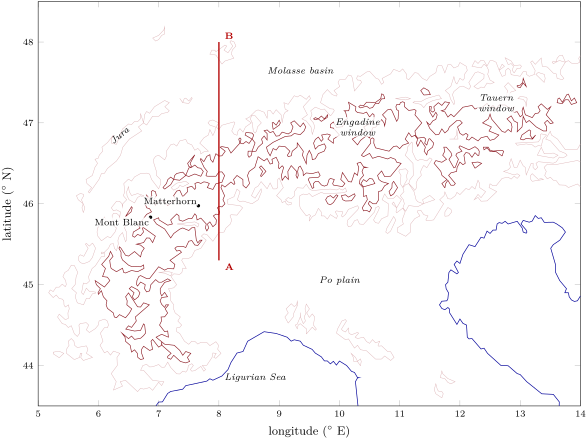
How can an ocean that has gone be known? By pieces of its floor that escaped subduction and were caught in the mountain belt.
Definition 13.2 (Ophiolite; Penrose ophiolite sequence)
An ophiolite is a distinctive assemblage of mafic to ultramafic rocks, a piece of oceanic lithosphere now found on land. The Penrose ophiolite sequence is the complete assemblage defined by a conference of geologists in 1972; from bottom to top:
- an ultramafic complex of harzburgite, lherzolite and dunite, usually with a deformation fabric acquired in the solid state;
- a gabbroic complex, ordinarily with cumulus textures;
- a mafic sheeted dyke complex;
- a mafic volcanic complex, commonly pillowed.
The Penrose definition was a consensus, criticised from the start, and still generally accepted. Its sequence is the layering of the oceanic crust and upper mantle met in the Year 1 volume: pillow lavas over sheeted dykes over gabbro over the mantle. Ophiolites, however, are not average ocean floor. Most abyssal crust, the crust of the wide oceans, is consumed by subduction; Coleman argued that the ophiolites of the Alpine and Cordilleran belts formed mainly at the spreading centres of small ocean basins or between island arcs, and that the Tethyan ones formed where continental crust thinned along passive margins until a small ocean opened.
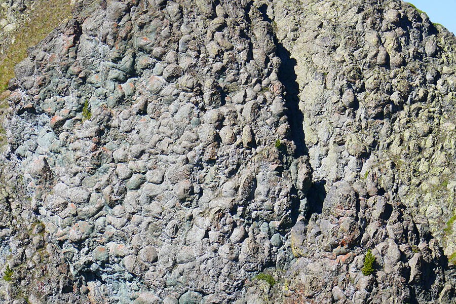
The Alpine ophiolites fit that picture. The units derived from the Piemont–Liguria ocean are relics of oceanic lithosphere and of mantle that had been brought up from beneath the thinned continent, the sub-continental mantle, and exposed on the sea floor. At the Chenaillet, in the Western Alps, the best preserved of them shows exposed mantle, gabbros and a famous sequence of pillow basalts, with no sedimentary cover. The photograph below shows them.
The ocean floor can be dated where its gabbros crystallised. Zircons from two metagabbros of the Zermatt–Saas ophiolite, below the Matterhorn, give and , and the manganese-rich sediments laid on the basalts are at most old: the floor of the Piemont–Liguria ocean was forming in the Jurassic, about ago.
13.2 Subducting an ocean, then a continent
An ocean closes by subduction. Some of its floor, though, ends up on top of a continent rather than beneath it, and some continents follow the ocean down.
Definition 13.3 (Obduction; continental subduction)
Obduction is the emplacement of a slab of oceanic lithosphere onto a continental margin, the ophiolite riding over the continent. Continental subduction is the descent of continental lithosphere, pulled by the oceanic slab attached to it, into a subduction zone after the ocean in front of it has been consumed.
Obduction happened in the Dinarides, south-east of the Alps: ophiolites of the Jurassic Vardar ocean, themselves of Middle Jurassic age, were thrust in the Late Jurassic onto an accretionary wedge and onto the margin of Apulia. It was long thought to have placed the Chenaillet ophiolite as well, because its rocks show only very low-grade Alpine metamorphism. A recent study found relics of lawsonite and omphacite in its gabbro and albitite, which put its Alpine peak at 10 to and 340 to : the weight of a nappe pile some 35 to thick. The authors conclude that the Chenaillet was subducted, not obducted, a reminder that the reading of an ophiolite rests on its metamorphic history as much as on its rocks.
The ocean goes down
In the Cretaceous the southern, Apulian margin of the Piemont–Liguria ocean became an active margin: its trench filled with shales and sandstones, now the calcareous schists called Bündnerschiefer or schistes lustrés. The eastern Alps also record an earlier collision, the closure of a gulf of another ocean, the Meliata, into Apulia, with a high-pressure peak at around : the Alps are the product of two orogenies, a Cretaceous one and a Tertiary one.
The Zermatt–Saas ophiolite went down to the eclogite facies of Chapter 10: its eclogites reached 550 to and 2.5 to , and peak pressure was reached between 48 and . One slice of it, at Lago di Cignana, holds coesite and microscopic diamonds in rocks that began as basalts and ocean-floor sediments; it reached about and , and its zircons date that deepest point at . Ocean floor born ago was subducted, at the age of 120 million years, to depths of or more, then came back.
The continent follows
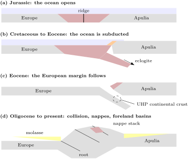
When the ocean had gone, Europe’s margin was dragged after it. The coesite-bearing quartzites of the Dora Maira massif, met in Chapter 11, are continental crust from the European side of the ocean that reached more than , about ago, and came back at the speed of plates. Dating the high-pressure rocks across the belt gives an order: the Apulian margin itself (the Sesia zone) in the Late Cretaceous, the ophiolites of the Piemont–Liguria ocean at about , the European continental crust in the late Eocene. Rubatto and colleagues read it as three episodes of subduction stepping in time from south-east to north-west, towards Europe.
Collision followed: the Valais ocean, the last oceanic strip, closed during the middle to late Eocene, and from then on continental crust was stacked on continental crust. The figure below sums up the sequence.
13.3 Nappes, klippen and windows
The pieces of ocean and continent were not piled up whole. They were scraped off as thin slices and carried far.
Definition 13.4 (Nappe; nappe stack)
A nappe is a large sheet of rock, often a few kilometres thick and tens of kilometres long, carried along a low-angle thrust or in the overturned limb of a large recumbent fold far from its place of origin; the rocks of a nappe are allochthonous, those that stayed in place autochthonous. A nappe stack is a pile of nappes in which the structurally higher nappes usually come from farther inside the orogen.
In the Alps the stacking order is the geography of the vanished ocean turned upside down, and the units are named by their origin (table below).
| unit (top to bottom) | origin and rocks |
|---|---|
| Austroalpine nappes | margin of Apulia north of the Periadriatic Line: basement and cover slices detached from their lower crust |
| Margna–Sesia nappes (Sesia zone, Dent Blanche) | fragments rifted off the outermost Apulian margin when the ocean opened |
| Upper Penninic nappes | Piemont–Liguria ocean: ophiolites, exhumed mantle, calcareous schists |
| Middle Penninic nappes | the Briançonnais ribbon continent |
| Lower Penninic nappes | Valais ocean: ophiolites and calcareous schists |
| Subpenninic nappes | European basement detached from its lower crust |
| Helvetic nappes | limestone-rich cover of the near European margin, detached from its basement |
| Southern Alps | Apulia south of the Periadriatic Line: a south-verging fold–thrust belt, mostly Miocene, 10 to thick |
The upper plate, Apulia, sits on top; beneath it come, in order, the far ocean, the Briançonnais, the near ocean and the European margin, the lowest units being those that were nearest Europe. Large folds that refolded the nappes after they were stacked sometimes upset the order, and some slivers, like the Briançonnais, wedge out along the belt.
Erosion then cuts the stack, and two shapes appear on a map.
Definition 13.5 (Klippe; tectonic window)
A klippe (plural klippen) is an isolated remnant of a nappe, left standing on the rocks beneath it when erosion has removed the rest of the sheet; it is surrounded by its basal thrust. A tectonic window is a hole eroded through a nappe, where the rocks beneath its basal thrust appear, surrounded by the nappe.
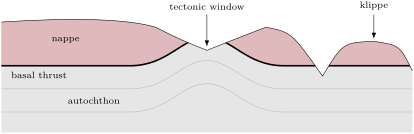
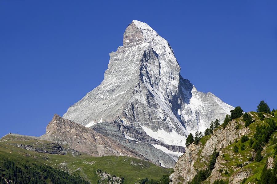
The Alps are full of both. The Matterhorn is a klippe: its summit belongs to the Dent Blanche thrust system, an outlier of Apulian rocks standing on top of the whole wedge, its gneisses and gabbros of Permian age resting on the ophiolites of the Zermatt–Saas nappe and the Combin zone, which rest in turn on the Monte Rosa and Grand St Bernard nappes of the European side (photograph below). At the northern front of the western Alps, cover nappes from far inside the belt form the Préalpes Romandes and the klippen of central Switzerland. In the eastern Alps two windows open through the Austroalpine lid: the Engadine window, where Valais ocean schists with blueschists appear beneath the last scraps of the Briançonnais, and the larger Tauern window, where the European margin and slices of the Alpine Tethys come out from under the Austroalpine nappes.
Detachments and the two skins
Nappes and thrust sheets move on surfaces of weakness.
Definition 13.6 (Décollement)
A décollement is a low-angle surface along which a sequence of rocks is detached from those beneath and slides over them, both sides deforming independently; it usually follows a weak layer such as evaporite or shale.
Definition 13.7 (Thin-skinned and thick-skinned tectonics)
Thin-skinned tectonics is deformation of a sedimentary cover detached from its basement along a basal décollement: the cover folds and thrusts while the basement beneath stays undeformed. Thick-skinned tectonics is deformation in which the basement is involved, cover and basement shortening together on faults that cut down into the basement.
Definition 13.8 (Fold–thrust belt)
A fold–thrust belt is a belt of folds and thrust faults that shortens the outer part of an orogen and propagates towards its foreland; thrusts step up from the décollement through the layers, and folds grow above them.
The Alps have both skins. The Helvetic nappes are a thin-skinned fold–thrust belt, the Mesozoic limestones of the near European margin detached from their basement. Their base is the Glarus thrust, where Permian red beds lie on Cenozoic flysch. In the Miocene, by contrast, basement blocks of the external massifs, shortened and thickened European basement (the Aar, Mont Blanc, Belledonne, Pelvoux and Argentera massifs), were thrust up with their cover: thick-skinned thrusting.
The Jura, the arc of ridges north-west of the Swiss plain, is the classic example of thin skin. In the late Miocene and Pliocene its Mesozoic cover was folded and thrust above a décollement in the weak Middle and Upper Triassic evaporites, while the basement beneath it, which continues from the external massifs under the Molasse basin, was not involved: on the classic reading, the push came from the distant external massifs. Seismology has since added a thick-skinned chapter. The earthquakes at Saint-Ursanne in 2000 had their source less than a kilometre down and a thrust mechanism, active shallow thrusting in the cover, while other studies find basement faults reactivated since the latest Pliocene. Whether the Jura is still detached from its basement is debated.
In the field — Reading a thrust contact
Between Flims and the Walensee in eastern Switzerland runs the Glarus thrust, one of the most prominent large low-angle thrusts of the Alps. Along it, Permian red beds, the Verrucano, lie above Cenozoic flysch, far older rocks resting on younger ones. Between them, a thin, strongly sheared band of limestone forms the contact: the Lochseiten limestone, on which the displacement, at least 30 to , was concentrated. In the nineteenth century Heim read the structure as two huge overturned folds facing each other; Escher von der Linth had read one overthrust, and the thrust reading prevailed. A geologist who meets such a contact checks three things: whether older rocks lie on younger ones, which no ordinary bedding can do; whether the layers on either side are cut off at the contact; and whether the contact itself is a band of sheared, recrystallised rock rather than a bedding plane.
13.4 Foreland basins: flysch and molasse
A mountain belt loads the plate it rides on, and the plate bends down in front of it.
Definition 13.9 (Foreland basin; flysch; molasse)
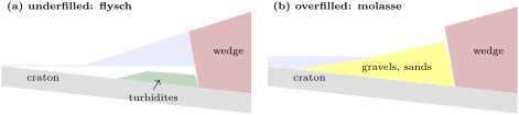
A foreland basin is an elongate sedimentary basin that forms between an orogen and the stable continent in front of it, where the plate is bent down by the load of the thrust wedge; it is deepest next to the thrust front and is itself progressively overthrust. Flysch is the deep-water fill of such a basin, chiefly turbidites of sandstone and shale deposited while the basin is underfilled. Molasse is its later shallow-marine and continental fill, chiefly conglomerates and sandstones from the eroding belt, deposited once the supply fills the basin.
The bending is elastic flexure of the lithosphere, treated in a Year 3 chapter; here only its effect on the basin matters. Sinclair described the early Alpine foreland basin, of Paleocene to Oligocene age, as an “underfilled trinity”: limestones on the continental side, hemipelagic mud in the middle, deep-water turbidites against the thrust front. As the thrusts advanced, the basin moved with them: across Switzerland its continental shoreline crept north-westwards at 8.5 to a year, and the basin migrated with an almost steady shape for at least over the European plate.
The north Alpine Molasse basin, which stretches from the Maritime Alps to Vienna, began to subside in the late Eocene. Lower Oligocene flysch, now found on top of the Helvetic nappes, records a last deep-water stage; from the late Oligocene to the late Miocene, rivers spread continental gravels and sands from the young mountains. The name is old: H.-B. de Saussure introduced molasse in 1779. The fill thickens towards the belt: in the Austrian sector, to more than at the thrust front, and elsewhere in the basin a single late Oligocene suite of river conglomerates is some thick. The southern part of the basin has been overridden: the Austrian outcrop belt, about wide, is less than a quarter of the basin’s former width. The overridden molasse itself is caught in the thrusts as the Subalpine Molasse, south-dipping slices of conglomerate along the northern rim of the belt.
South of the Alps, the Po plain lies on the little-deformed Adriatic foreland of the Southern Alps. Its youngest, Pliocene and Pleistocene, sediments partly cover Alpine structures unconformably and are partly deformed by the last thrusts of the Southern Alps and of the Apennines.
13.5 Reading the history: sections and geophysics
A map shows where the units are; a cross-section shows how they lie beneath, and it can be tested.
Definition 13.10 (Balanced cross-section)
A balanced cross-section is a cross-section of deformed rocks, drawn parallel to the direction of transport, that can be restored to a geologically reasonable undeformed state without gaining or losing rock: the lengths of marker beds and the areas of rock units in the section are conserved between the deformed and the restored states.
The restoration is anchored by pin lines, lines across the layers at the ends of the section, chosen where the rocks did not slip past one another.
Proposition 13.11 (Line-length and area balance)
Between two pin lines a distance apart in the deformed state, let a marker bed have a length measured along the bed, and let a layer of original thickness have a cross-sectional area . If length and area are conserved in the plane of the section,
- the bed was long before deformation, the shortening is and the shortening distance is ;
- the restored length of the layer is ;
- if a marker horizon lay at a depth above a flat décollement, the area of rock raised above the marker’s original level, its excess area , equals ; hence .
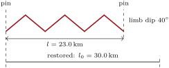
Proof. (1) A bed that neither stretches nor shortens along its length keeps it; the shortening is the fraction of length lost, as at school. (2) Before deformation the layer is a strip of length and thickness , of area , and the area is conserved. (3) Before deformation, the rock between the marker’s level and the décollement filled a strip long and thick. After it, between the pin lines, the same rock fills a strip long from the décollement up to the marker’s original level, of area , plus the excess area pushed above that level. Conservation gives , so . The relation gives the depth of a hidden décollement from a measured excess area and shortening. ∎
Method 13.12 (Restoring a section)
- Choose a section parallel to the transport direction and two pin lines where there was no slip between layers.
- Measure each marker bed along its length between the pins, counting every part repeated by a thrust.
- Lay the beds out flat at their measured lengths, keeping the order of the layers, and redraw the faults on the restored section: their cut-offs must line up, without gaps or overlaps.
- Compare: beds of the same thrust sheet must restore to the same length; the areas of the layers, divided by their thicknesses, must give the same lengths too. A section that fails is not admissible as drawn.
Balancing is a test of a section, not a proof of it, and its assumptions matter. In the Jura near the Chasseral, line-length balancing of the top of the Jurassic gives of displacement, but area balancing and forward modelling give : the extra was carried along a second, upper detachment in the Jurassic shales and passed on to folds further north. One marker bed had missed half of the movement. The same study weighed, and did not need, two other readings common in the Jura: basement highs pushing up the folds, and anticline cores thickened by Triassic evaporites flowing into them, a process that defeats area balance, since the evaporite layer no longer keeps its thickness.
How much shortening?
Applied to whole transects, balancing gives the bulk shortening of the belt, and the answers differ with the assumptions. Across the Central Alps, along the NFP-20 transect, estimates of collisional shortening have been about in earlier work, in a 2015 compilation and in a 2021 review; adding the dextral slip on the Periadriatic Line, which moved Apulia sideways along the belt, raises the bulk convergence to between 206 and , depending on how much slip is assumed. In the Western Alps the estimates range from 124 to . Every one of them is a sum of restored pieces, each with its own pin lines and its own guesses about what erosion and subduction removed.
What the geophysics sees
Sections at depth rest on geophysics. Deep seismic reflection profiles have been shot across the belt (ECORS–CROP in the Western Alps, NFP-20 West and East in Switzerland, TRANSALP in the east), and dense networks of seismometers now map the Moho from receiver functions, the conversions of teleseismic P waves into S waves at the base of the crust. The AlpArray map, built from more than a hundred thousand receiver functions, finds the Moho at about , typical of continents, around the belt, and at 55 to beneath the Alps; the European Moho dips gently from about in the north-west to about under the range. The schematic section below sums up how the NFP-20 profiles across the Central Alps are read.
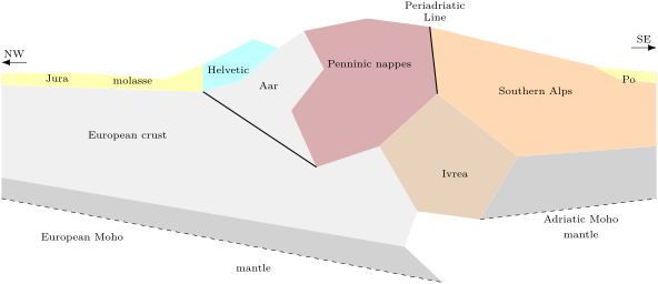
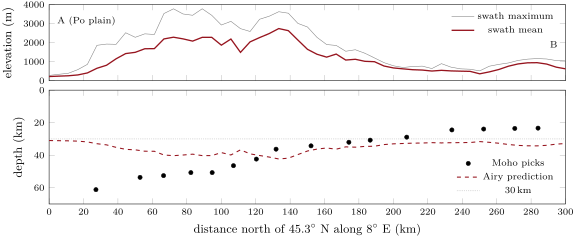
The profile above confronts the root with Airy’s model of the Year 1 volume. Under the highest part of the profile, where the swath-mean relief reaches at N, a local Airy root would put the Moho at ; it is observed at . About a hundred kilometres further south, at the edge of the Po plain, where the mean relief is only , the observed Moho is the deepest of the profile, . The root is not under the peaks: it is displaced towards Apulia. Over the stretch where picks exist, its cross-section, measured below , is about , against about for the Airy roots of the relief above it. Local compensation of the present topography does not explain the root. Pfiffner and colleagues point to an extra load: the Ivrea body, a wedge of Adriatic mantle and lower crust within the belt, which helped bend the European plate down.
Gravity tells the same story in another way. The pan-Alpine Bouguer anomaly map shows an Alpine gravity low of to along the range, deepest in the Central Alps, from the light crust of the thickened root; a Po basin low of about to ; and, between the Western Alps and the Po plain, the narrow Ivrea gravity high, up to , where that dense lower crust and mantle come close to the surface.
13.6 A timeline of the Alps
Gathering the dates of this chapter gives the belt’s history in one table (table below).
| time | event |
|---|---|
| Middle Jurassic | the Piemont–Liguria ocean opens; its gabbros crystallise at |
| earliest Cretaceous | the Valais ocean opens north of the Briançonnais |
| about | high-pressure peak of the Cretaceous orogeny in the eastern Alps |
| Late Cretaceous | the Apulian margin (Sesia zone) is subducted; the Apulian margin of the ocean is active |
| 48 to | the Zermatt–Saas ocean floor reaches its deepest point, coesite and diamond at Lago di Cignana |
| middle to late Eocene | the Valais ocean closes; the Molasse basin starts to subside |
| continental crust of the Dora Maira at ultrahigh pressure | |
| Oligocene and Miocene | the Glarus thrust; molasse gravels fill the northern foreland (late Oligocene to late Miocene) |
| Miocene | thick-skinned uplift of the external massifs; the Southern Alps thrust southwards |
| late Miocene to Pliocene | thin-skinned folding of the Jura |
| today | levelling shows relative rock uplift of up to a year in the core of the Central Alps |
The last line is not the end of convergence. Repeated levelling across the Central Alps gives relative rock uplift from about a year north of the Jura to a year in the core of the range, while GPS measurements suggest that the Central Alps are not converging today. Champagnac and colleagues read the uplift as the isostatic rebound of a crust being unloaded by erosion: the mountains rise because they are worn down.
Exercises
Data for the exercises: , .
Exercise 13.1 ★
In a cross-section, a limestone bed measured along its folds between two pin lines is long; the pin lines are apart. (a) Using Proposition 13.11, compute the shortening and the shortening distance . (b) What has to be true of the bed for the answer to hold?
Solution
Solution of Exercise 13.1.
(a) , that is ; . (b) The bed must have kept its length (no stretching or thinning along it), the section must be parallel to the transport direction, and the pin lines must mark places where the layers did not slip past each other.
Exercise 13.2 ★
On a geological map, (a) an oval patch of gneiss long lies on Jurassic limestone, its boundary a thrust that dips inwards, beneath the gneiss, all round; (b) an elongate area of Cretaceous shale is surrounded by gneiss, along a thrust that dips outwards, beneath the gneiss, all round. Name each structure and say what erosion has done in each case.
Solution
Solution of Exercise 13.2.
(a) A klippe: the gneiss is an isolated remnant of a nappe resting on its autochthon; erosion has removed the rest of the sheet all round it. (b) A tectonic window: erosion has cut through the gneiss nappe and exposed the younger rocks beneath its basal thrust, which therefore dips away from the window on every side.
Exercise 13.3 ★
(a) List the four units of the Penrose ophiolite sequence from bottom to top, and match each with a layer of the oceanic crust or mantle. (b) The Chenaillet ophiolite shows exposed mantle, gabbro and pillow basalts, and no sedimentary cover. Which Penrose unit does this list leave out? (c) Why do ophiolites not give a fair sample of the floor of the wide oceans?
Solution
Solution of Exercise 13.3.
(a) Ultramafic complex (the upper mantle); gabbroic complex (the lower oceanic crust); sheeted dyke complex (the middle crust); volcanic complex, pillowed (the upper crust). (b) The sheeted dyke complex. (c) Most crust of the wide oceans is consumed by subduction; the ophiolites that survive on land formed mostly in small ocean basins or between island arcs, the Tethyan ones where a continent thinned until a small ocean opened.
Exercise 13.4 ★
On the way up the Matterhorn from the south, a climber crosses in turn the Monte Rosa and Grand St Bernard nappes, the Zermatt–Saas ophiolites, the Combin zone and the gneisses of the Dent Blanche thrust system. (a) Give the domain of origin of each. (b) Which plate was the upper plate during subduction? (c) Why is this order a general rule in the nappe stack, and what can break it?
Solution
Solution of Exercise 13.4.
(a) Monte Rosa and Grand St Bernard nappes: the European side (the Briançonnais and the European passive margin); Zermatt–Saas and Combin zone: the Piemont–Liguria ocean; Dent Blanche system: the margin of Apulia. (b) Apulia, which ends on top. (c) The upper plate is not subducted, and the slices scraped off the lower plate stack beneath it in the order the lower plate arrived: far ocean first, near margin last and lowest. Later folding of the pile, or out-of-sequence thrusts, can upset the order.
Exercise 13.5 ★★
The Central Alps carry a Bouguer anomaly of about . (a) Using the Bouguer slab of the Year 1 volume, , find the thickness of an infinite slab of density deficit (crust replacing mantle) that gives this anomaly. (b) The receiver functions show a root of about below a crust. What anomaly would an infinite slab that thick give? (c) Why is the observed anomaly smaller?
Solution
Solution of Exercise 13.5.
(a) ; . (b) , about . (c) The root is not an infinite slab: it is a body some tens of kilometres deep and only about as wide as the belt, so it pulls less on a point at the surface than a slab of the same thickness extending to infinity would; dense bodies such as the Ivrea zone add positive anomalies, and the density contrast at depth may be smaller than assumed.
Exercise 13.6 ★★
Gabbros of the Zermatt–Saas ophiolite crystallised at ; the ophiolite reached its deepest point at , at . (a) How old was the oceanic lithosphere when it was subducted? (b) Convert the pressure to depth with a mean overburden density of , then . (c) Compare with the “more than ” quoted for this rock.
Solution
Solution of Exercise 13.6.
(a) . (b) : ; . (c) “More than ” lies inside this range: the depth depends on the mean density chosen for the overburden as much as on the pressure.
Exercise 13.7 ★★
A bed is folded into chevrons whose straight limbs all dip at the angle . (a) Show that the shortening is . (b) What limb dip gives shortening? (c) What shortening do limbs dipping and give? Check the first against the chevron figure of the section on balancing.
Solution
Solution of Exercise 13.7.
(a) A limb of length dipping at spans horizontally; all limbs have the same dip, so and . (b) : . (c) , as in the chevron figure; .
Exercise 13.8 ★★
A cover thick is folded and thrust above a flat décollement. Between pin lines now apart, its cross-sectional area is . (a) Find its restored length, and . (b) Compute the excess area and the depth of the décollement below the original top of the cover. (c) Is the result consistent?
Solution
Solution of Exercise 13.8.
(a) ; ; . (b) ; . (c) Yes: the décollement lies at the base of the cover, below its top; the cover is detached on its base.
Exercise 13.9 ★★
Along the E profile of this chapter, the swath-mean elevation is at N, where the Moho is picked at , and at N, where it is picked at . (a) With a reference crust, and , compute the Airy Moho depth at both places. (b) Compare with the picks. (c) What does the comparison say about how the Alpine root is held?
Solution
Solution of Exercise 13.9.
(a) The Airy root is : at N, , a Moho at ; at N, , a Moho at . (b) Under the high ground the Moho is shallower than Airy predicts; under the edge of the Po plain it is deeper. (c) The root is not compensated locally: it is displaced towards the south and larger than the relief requires. The plate bends as a whole under the loads on it (the regional support of a Year 3 chapter), and one of those loads, the Ivrea body, is not topography at all.
Exercise 13.10 ★★★
In the Chasseral section of the Jura, line-length balancing of the top of the Jurassic gives of displacement; area balancing and modelling give , of which was carried along an upper detachment in Middle Jurassic shales. (a) What fraction of the displacement did the top-Jurassic bed record? (b) Show that the numbers add up, and explain why the upper bed misses part of the movement. (c) What general lesson does this give for balancing with a single marker bed?
Solution
Solution of Exercise 13.10.
(a) : less than half. (b) . The top of the Jurassic lies above the upper detachment; the carried along that detachment passed beneath the folds of the section and was spent in structures further north, so the upper bed never shortened by that amount within the section. (c) A single marker bed records only the shortening of the layers it belongs to; every detachment above or below it can carry displacement in or out of the section. Balance several beds, and check with areas.
Exercise 13.11 ★★★
Across the Central Alps, about of north-directed shortening has been estimated, and the Periadriatic Line has an east–west dextral offset of about , perhaps 50, perhaps 150. (a) Add the two as perpendicular vectors and give the bulk convergence for each offset. (b) What angle does the convergence make with the north–south direction for an offset of ? (c) Why does the choice of offset matter more than the third significant figure of the shortening?
Solution
Solution of Exercise 13.11.
(a) For an offset of , ; for , ; for , . (b) from north–south, a convergence line close to the NE quoted by Rosenberg and colleagues. (c) The offset is uncertain by , which moves the bulk convergence by about either way; the third figure of the result is far below that uncertainty.
Exercise 13.12 ★★★
The Swiss part of the Alpine foreland basin migrated at least north-westwards over Europe, its shoreline advancing at 8.5 to a year. (a) Over what range of durations did the migration last? (b) In the Austrian sector, the present outcrop belt, about wide, is less than a quarter of the basin’s former width. What was the least former width, and how much of the basin is hidden under the thrusts? (c) Why can a foreland basin never be fully preserved?
Solution
Solution of Exercise 13.12.
(a) to ( divided by gives millions of years). (b) More than ; at least of the basin is now under the Alpine thrusts or has been eroded. (c) The basin forms in front of the thrust wedge and migrates with it: its inner part is always being overridden by the thrusts that load it, and its oldest fill is caught in the thrusts, as the Subalpine Molasse is.
Problem 13.1
Weekend problem — restoring the section
An Alpine-type orogen is crossed by a model section (an invented geometry, the book’s own, labelled as a model) made of five domains, from the foreland to the far side: a foreland fold–thrust belt, wide today; an external nappe stack, ; a basement massif, ; an internal zone of continental nappes and ophiolites, ; and a south-verging retro-wedge, (figure below). Lengths are in kilometres throughout.

Part I — Line-length balance of the foreland belt. Between its two pin lines, apart, the top of the main limestone is made of ten straight segments (horizontal extent , dip), listed from the foreland; in addition, a thrust sheet covers a flat stretch of the same bed, long, which is repeated beneath it.
| segment | 1 | 2 | 3 | 4 | 5 | 6 | 7 | 8 | 9 | 10 |
|---|---|---|---|---|---|---|---|---|---|---|
| () | 8.0 | 3.0 | 3.0 | 5.0 | 2.5 | 2.5 | 6.0 | 4.0 | 4.0 | 10.0 |
| dip () | 0 | 35 | 35 | 0 | 50 | 50 | 10 | 40 | 40 | 5 |
- Compute the length along the bed of segments 2, 5 and 8.
- Compute the total length of the bed between the pin lines, including the repeated stretch.
- Why must the stretch hidden under the thrust sheet be counted?
- Compute the shortening and the shortening distance of the foreland belt.
- The base of the limestone, measured the same way, is long. By how much, and by what percentage, do the two beds disagree? Is the section acceptable?
- What would a length of for the base have meant?
Part II — Area balance and the décollement. The cover between the décollement and the top of the limestone was thick before deformation; its area between the pin lines is measured as .
- Compute the restored length of the cover from its area.
- Compare with the line-length result of question 2.
- Compute the excess area, raised above the cover’s original top.
- Deduce the depth of the décollement below that level, and compare it with the cover thickness.
- Had the area been , what restored length would it give? Which process, named in the Jura, could make the area and the line length disagree that way?
- Why is this belt thin-skinned, and what should the top of the basement look like beneath it?
Part III — The external nappes and their pace. The marker bed of the three external nappes restores to 22, 18 and ; the stack now spans . In the basement massif, the top of the basement restores to against today. The foreland belt deformed between 11 and , the nappes between 30 and .
- Compute the restored length of the nappe stack and its shortening distance.
- Compute its shortening and compare it with that of the foreland belt.
- Compute the shortening of the basement massif. What kind of tectonics is this?
- Compute the mean shortening rates of the foreland belt and of the nappes, in millimetres a year.
- In which direction did deformation migrate through the section? Is this the order of the Alps?
- Add up the shortening of the three external domains.
Part IV — The internal zone, the ocean and the whole section. Ophiolite slivers in the internal zone restore to . Suppose that the ocean was subducted from 85 to at a mean rate of a year. The continental nappes of the internal zone restore to against today, and the marker bed of the retro-wedge to against .
- What length of oceanic lithosphere was subducted?
- Give a minimum width for the ocean.
- Why is it only a minimum?
- Compute the shortening of the internal zone and of the retro-wedge.
- Add up the collisional shortening of the five domains, and compare it with the estimates for the Central Alps in this chapter.
- Crustal check: restore the section to its full width with a crust, and compare the crustal area with today’s, a mean of over the present . What fraction of the crust is missing from the present section, and where did it go? Give the total collisional shortening across the section, rounded to the kilometre.
Solution
Solution of Problem 13.1.
Part I.
1. ; ; .
2. ; with the repeated stretch, .
3. The bed beneath the thrust sheet is the same bed, carried under the sheet by the thrust: before thrusting it lay in line with the rest. Leaving it out would restore the bed too short.
4. , that is ; .
5. , : within the precision of the measurement; the section is acceptable.
6. , : the two beds of one sheet cannot restore to such different lengths. The section would not be admissible as drawn: a structure missing or misdrawn, a pin line in the wrong place, movement out of the plane of the section, or a detachment between the two beds.
Part II.
7. .
8. It differs from by : line length and area agree.
9. .
10. , equal to the of the cover to the precision of the data: the décollement is the base of the cover.
11. , more than the line length. Thickening of the evaporites at the base of the cover, flowing into the cores of anticlines, adds area without adding length; area balance with a constant thickness then fails.
12. The cover moved on a décollement at its base and the basement was not involved. Beneath the belt the top of the basement should run flat or dip gently and evenly, unbroken by the thrusts above it.
Part III.
13. ; .
14. , against in the foreland belt: the nappes are far more shortened.
15. (). The basement itself is shortened: thick-skinned tectonics.
16. Foreland belt , that is a year; nappes a year.
17. The nappes (30 to ) deformed before the foreland belt (11 to ): deformation migrated outwards, towards the foreland. This is the order of the Alps: the Glarus thrust in the Oligocene and Miocene, the external massifs in the Miocene, the Jura in the late Miocene and Pliocene.
18. .
Part IV.
19. .
20. .
21. Only what is preserved or inferred is counted: parts of the ocean may have been subducted before or faster than the mean rate, ophiolite slices may have been eroded or carried out of the section, and convergence oblique to the section brings in ocean floor the section does not see.
22. Internal zone (); retro-wedge ().
23. ; within the range of the estimates for the Central Alps, about 125 to of collisional shortening (before adding strike slip).
24. Restored width ; restored crust ; present crust . Missing: , of the restored crust; it has been eroded (and shed into the foreland basins) or subducted with the lower crust into the mantle. Without those losses the crust would be thick on average. The total collisional shortening across the section is .