书籍暂未推出简体中文版——当前显示英文版。

University Earth and Space Sciences — Year 2 · 本科二年级

25Orbital Forcing and the Ice Ages

Over the last million years the shape of the Earth’s orbit has changed the sunlight received by the whole planet in a year by less than two parts in a thousand: between $340.00$ and $340.54\,\mathrm{W}\,\mathrm{m}^{-2}$ at the top of the atmosphere. Over the same million years the daily-mean sunshine of mid-July at $65{}^{\circ}$ N has swung between about 388 and $500\,\mathrm{W}\,\mathrm{m}^{-2}$ , by more than a quarter. The ice ages followed the second number, not the first. This chapter computes both from the elements of the Earth’s orbit, and asks how sunlight at one latitude in one season can pace the growth and decay of ice sheets that cover continents.

You already know

From the physics books: the ellipse, its semi-major axis $a$ and eccentricity $e$ , Kepler’s laws. From the Year 1 volume: the ecliptic and the obliquity $\varepsilon$ , the Sun’s declination $\delta$ with $\sin\delta = \sin\varepsilon\sin\lambda$ ( $\lambda$ the Sun’s true longitude, counted along the ecliptic from the vernal equinox), the tropical year, the daily-mean insolation

\bar Q = \frac{S_0}{\pi}\left(\frac{a}{r}\right)^{2}\bigl(h_0\sin\varphi\sin\delta + \cos\varphi\cos\delta\sin h_0\bigr),\qquad \cos h_0 = -\tan\varphi\tan\delta ,

and its global and annual mean, $S_0/(4\sqrt{1 - e^2})$ . From the school volumes: the glacial cycle and the Last Glacial Maximum; radiative forcing. From earlier chapters: the ice–albedo feedback (Definition 18.8); the benthic stack, the EPICA Dome C record and age models (Chapter 24).

25.1 The orbit and its three elements

The Earth’s orbit is an ellipse with the Sun at one focus. The planets, Jupiter and Saturn above all, slowly deform it and turn it in its plane; the pull of the Sun and the Moon on the equatorial bulge makes the axis of rotation wobble like a top. Three quantities describe what matters for sunlight: how elongated the ellipse is, how tilted the axis is, and where along the orbit the seasons fall.

Definition 25.1 (Longitude of perihelion; climatic precession)

The longitude of perihelion $\varpi$ is the angle, measured in the plane of the orbit from the direction of the vernal equinox, between that direction and the direction of the perihelion seen from the Sun; it is counted from the moving equinox, so it changes with both the wobble of the axis and the turning of the orbit. The climatic precession is the quantity $e\sin\varpi$ , also called the precession index.

The Earth’s orbit seen from the north side, with the eccentricity exaggerated to 0.3 and today’s longitude of perihelion,

\varpi = 101.4{}^{\circ}

. The Earth moves anticlockwise (arrow); the points mark its position at the equinoxes and solstices. The perihelion falls a few days after the December solstice, the aphelion a few days after the June solstice. Schematic.

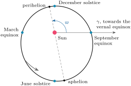
Seen from the Earth, the Sun moves along the ecliptic, and its true longitude $\lambda$ is the angle from the vernal equinox: $\lambda = 90{}^{\circ}$ at the June solstice, $270{}^{\circ}$ at the December solstice. The Earth is at perihelion when the Sun is in the direction opposite to the perihelion, at $\lambda = \varpi + 180{}^{\circ}$ ; today $\varpi = 101.37{}^{\circ}$ and the perihelion falls at $\lambda = 281.37{}^{\circ}$ , about eleven days after the December solstice, on or about 3 January.

Definition 25.2 (Milankovitch parameters)

The Milankovitch parameters are the three orbital quantities that set the distribution of sunlight over the Earth through the seasons and the latitudes: the eccentricity $e$ , the obliquity $\varepsilon$ and the climatic precession $e\sin\varpi$ . The Milankovitch theory states that their slow variations pace the growth and decay of the Quaternary ice sheets, through the summer insolation at high northern latitudes.

Each parameter varies with its own rhythms. The eccentricity has main periods near $95\,000$ , $99\,000$ , $124\,000$ and $131\,000$ years, which combine into a cycle of about $100\,000$ years, and a period of $405\,000$ years, the most stable of all; over the last million years it ranged from $0.0046$ to $0.0565$ , and today, at $0.0172$ , it is slowly decreasing. The obliquity varies with a main period of $40\,978$ years, between $22.1{}^{\circ}$ and $24.5{}^{\circ}$ over the last million years; at $23.44{}^{\circ}$ it is decreasing, past its last maximum about $10\,000$ years ago. The axis wobbles round in about $25\,770$ years, while the orbit turns in about $112\,000$ ; together they move the perihelion through the seasons with main periods near $19\,000$ , $22\,400$ and $23\,700$ years.

The three Milankovitch parameters over the last million years: (a) the eccentricity; (b) the obliquity; (c) the climatic precession, whose envelope is the eccentricity. Data: Berger and Loutre (1991), NOAA NCEI Paleoclimatology, as fetched on 23 October 2026.

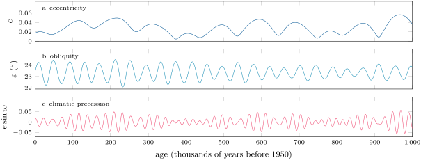
The climatic precession swings fast, but only as far as the eccentricity lets it: when the orbit is nearly circular, as $400\,000$ years ago, it hardly matters where the perihelion falls. The figure shows it plainly: the envelope of panel (c) is panel (a).

25.2 Sunlight from the orbit

The daily-mean insolation recalled above needs one more ingredient: the distance of the Sun on a given day.

Proposition 25.3 (Distance and the Sun’s longitude)

When the Sun’s true longitude is $\lambda$ , the Earth–Sun distance is

\frac{r}{a} = \frac{1 - e^2}{1 - e\cos(\lambda - \varpi)} .

At the June solstice ( $\lambda = 90{}^{\circ}$ ), to first order in $e$ , $(a/r)^2 \approx 1 - 2e\sin\varpi$ ; at the December solstice, $(a/r)^2 \approx 1 + 2e\sin\varpi$ .

Proof. On an ellipse with the Sun at a focus, $r/a = (1 - e^2)/(1 + e\cos v)$ , where the true anomaly $v$ is the angle at the Sun from the perihelion to the Earth. The Earth is seen from the Sun in the direction opposite to that of the Sun seen from the Earth, so its longitude seen from the Sun is $\lambda + 180{}^{\circ}$ , and $v = \lambda + 180{}^{\circ} - \varpi$ , $\cos v = -\cos(\lambda - \varpi)$ . At $\lambda = 90{}^{\circ}$ , $\cos(\lambda - \varpi) = \sin\varpi$ and $(a/r)^2 = (1 - e\sin\varpi)^2/(1 - e^2)^2 = 1 - 2e\sin\varpi + O(e^2)$ ; at $\lambda = 270{}^{\circ}$ the sign changes. ∎

The climatic precession is therefore the right index: it measures how much nearer to the Sun, or farther, the Earth is at the June solstice. When $e\sin\varpi$ is large and positive, as today and much more so $116\,000$ years ago, the northern summer falls near aphelion and is weak; when it is large and negative, as about $10\,000$ years ago, the northern summer falls near perihelion.

Example 25.4 (The June sun at $65{}^{\circ}$ N, today)

Today $e = 0.017236$ , $\varpi = 101.37{}^{\circ}$ , $\varepsilon = 23.446{}^{\circ}$ , and the tables use $S_0 = 1360\,\mathrm{W}\,\mathrm{m}^{-2}$ . At the June solstice $\delta = \varepsilon$ ; at $\varphi = 65{}^{\circ}$ , $\cos h_0 = -\tan65{}^{\circ}\tan23.446{}^{\circ} = -0.9301$ , so $h_0 = 158.44{}^{\circ} = 2.7654\,\mathrm{rad}$ : the Sun is up for $2 \times 158.44/360 \times 24 = 21.1$ hours. The bracket of the insolation formula is $2.7654 \times 0.9063 \times 0.3979 + 0.4226 \times 0.9174 \times 0.3674 = 1.1397$ , and at the mean distance $\bar Q = 432.90 \times 1.1397 = 493.4\,\mathrm{W}\,\mathrm{m}^{-2}$ . The distance factor is $(a/r)^2 = 0.9671$ , so $\bar Q = 477.1\,\mathrm{W}\,\mathrm{m}^{-2}$ .

Kepler’s second law adds a twist. Near aphelion the Earth moves more slowly: the season that falls there is weaker but lasts longer. Northern summers are today about 4.5 days longer than northern winters, and springs about three days longer than autumns.

Proposition 25.5 (Annual means do not depend on precession)

The energy received per unit area at the top of the atmosphere between two given longitudes of the Sun does not depend on $\varpi$ , and the annual-mean insolation at any latitude is that of a circular orbit of radius $a$ multiplied by $1/\sqrt{1 - e^2}$ . At a pole the annual mean is

\bar Q_{\text{pole}} = \frac{S_0\sin\varepsilon}{\pi\sqrt{1 - e^2}} ,

which grows with the obliquity.

Proof. By Kepler’s second law the radius sweeps area at the constant rate $\pi ab/T$ , and the area swept while the Earth turns by $\mathrm d\lambda$ is $\frac12 r^2\,\mathrm d\lambda$ , so $\mathrm dt = T r^2\,\mathrm d\lambda/(2\pi ab)$ , with $b = a\sqrt{1 - e^2}$ . The insolation at a given latitude and longitude of the Sun is $(a/r)^2$ times its value $Q_a(\lambda)$ at the distance $a$ , so the energy received is $\int Q_a(\lambda)(a/r)^2\,\mathrm dt = \frac{T}{2\pi\sqrt{1 - e^2}}\int Q_a(\lambda)\,\mathrm d\lambda$ : the distance has cancelled, and with it $\varpi$ . Over the whole year, $\lambda$ runs through $360{}^{\circ}$ and the mean is $\frac{1}{2\pi\sqrt{1-e^2}}\int_0^{2\pi} Q_a\,\mathrm d\lambda$ . At the North Pole $Q_a = S_0\sin\delta = S_0\sin\varepsilon\sin\lambda$ for $0 < \lambda < \pi$ and 0 otherwise; the integral is $2S_0\sin\varepsilon$ . ∎

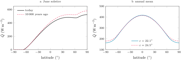
Precession moves sunlight from one season to another, never in or out of a year; eccentricity changes the yearly total by a factor $1/\sqrt{1 - e^2}$ , at most $0.16\,\%$ over the last million years; obliquity moves sunlight between latitudes, raising the annual mean at the poles and lowering it slightly at the equator. Only the seasonal and latitudinal pattern changes much, and that is what the figure below shows.

(a) Daily-mean insolation at the June solstice, today and 10\,000 years ago, when the northern summer fell near perihelion and the obliquity was larger: about 50\, W\, m-2 more in the northern high latitudes. (b) Annual-mean insolation for the two extreme obliquities of the last million years, with today’s eccentricity: a larger tilt sends more sunlight to the poles and slightly less to the tropics. Computed from the orbital elements with S_0 = 1360\, W\, m-2. — (a) Daily-mean insolation at the June solstice, today and $10\,000$ years ago, when the northern summer fell near perihelion and the obliquity was larger: about $50\,\mathrm{W}\,\mathrm{m}^{-2}$ more in the northern high latitudes. (b) Annual-mean insolation for the two extreme obliquities of the last million years, with today’s eccentricity: a larger tilt sends more sunlight to the poles and slightly less to the tropics. Computed from the orbital elements with $S_0 = 1360\,\mathrm{W}\,\mathrm{m}^{-2}$ .

25.3 Computing the insolation curve

The insolation curve that Milankovitch built is now a routine calculation. The orbital elements of the past are computed by integrating the motions of the planets; tabulated every thousand years, they are the input. For each age, the method below gives the insolation at any latitude and season.

Method 25.6 (Insolation of the past)

Read $e$ , $\varpi$ and $\varepsilon$ for the age wanted.
Choose the season by the Sun’s true longitude $\lambda$ : $90{}^{\circ}$ for the June solstice; the tables’ mid-July corresponds to $\lambda = 120{}^{\circ}$ .
Compute $\delta$ from $\sin\delta = \sin\varepsilon\sin\lambda$ , and the hour angle of sunset $h_0$ at the latitude $\varphi$ (polar day or night if $|\tan\varphi\tan\delta| > 1$ ).
Compute the distance factor $(a/r)^2$ with Proposition 25.3.
Multiply: $\bar Q = (S_0/\pi)(a/r)^2(h_0\sin\varphi\sin\delta + \cos\varphi\cos\delta\sin h_0)$ .

Applied to the 1001 ages of the last million years, the method reproduces the tabulated mid-July insolation at $65{}^{\circ}$ N to within $0.012\,\mathrm{W}\,\mathrm{m}^{-2}$ , the rounding of the tables, and the tabulated June values at the present day exactly. The tables put the origin of time at 1950.

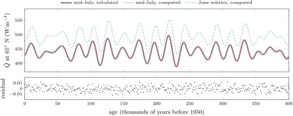
Top: daily-mean insolation at 65 N over the last 400\,000 years, mid-July as tabulated by Berger and Loutre (grey, wide) and as computed by the method above (red), and at the June solstice (blue, dashed). Bottom: computed minus tabulated mid-July values, in W\, m-2. — Top: daily-mean insolation at $65{}^{\circ}$ N over the last $400\,000$ years, mid-July as tabulated by Berger and Loutre (grey, wide) and as computed by the method above (red), and at the June solstice (blue, dashed). Bottom: computed minus tabulated mid-July values, in $\mathrm{W}\,\mathrm{m}^{-2}$ .

Two features stand out. The curve is dominated by the climatic precession, with peaks some $20\,000$ years apart whose height swells and shrinks with the eccentricity; the obliquity adds a slower modulation. And the swings are large: over the last $800\,000$ years the mid-July value ranged from 388 to $497\,\mathrm{W}\,\mathrm{m}^{-2}$ .

25.4 Milankovitch theory and the glacial cycles

History — Sunshine at sixty-five degrees north

Milutin Milankovitch, born in 1879, built a mathematical theory of climate from the seasonal and latitudinal variations of sunlight. Combining the three orbital variations, he computed the insolation of the latitudes and the corresponding surface temperatures for $600\,000$ years before 1800. At the suggestion of the climatologist Köppen he chose the summer insolation at $65{}^{\circ}$ N as the decisive quantity: the great ice sheets had grown near that latitude, and cool summers melt less of the winter’s snow, so that snow accumulates from year to year. He thought the obliquity the most important of the three parameters. For about fifty years the theory was largely ignored; Milankovitch died in 1958. In 1976 Hays, Imbrie and Shackleton found in deep-sea sediments of the last $450\,000$ years spectral peaks of climate variability at about $23\,000$ , $42\,000$ and $100\,000$ years, the periods of precession, obliquity and eccentricity, and concluded that changes in the Earth’s orbit are the fundamental cause of the Quaternary ice ages.

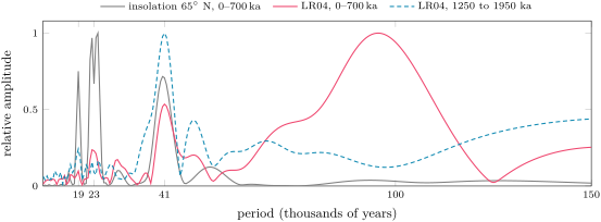
The figure below repeats their test on the records of Chapter 24. It compares the amplitude spectra, the strength of each period, of the $65{}^{\circ}$ N July insolation and of the benthic stack, in two windows of $700\,000$ years.

Amplitude spectra, each scaled to its own maximum, of the mid-July insolation at 65 N over the last 700\,000 years and of the LR04 benthic stack over the same window and over 1\,250\,000 to 1\,950\,000 years ago (trend removed, tapered). The insolation has its power at the precession periods, near 19 to 24 thousand years, and at the obliquity period; the recent ice volume peaks near 100\,000 years, where the insolation has almost nothing; the older ice volume peaks at 41\,000 years. — Amplitude spectra, each scaled to its own maximum, of the mid-July insolation at $65{}^{\circ}$ N over the last $700\,000$ years and of the LR04 benthic stack over the same window and over $1\,250\,000$ to $1\,950\,000$ years ago (trend removed, tapered). The insolation has its power at the precession periods, near 19 to 24 thousand years, and at the obliquity period; the recent ice volume peaks near $100\,000$ years, where the insolation has almost nothing; the older ice volume peaks at $41\,000$ years.

Glacials, interglacials and terminations

Definition 25.7 (Glacial period; interglacial; glacial termination)

In the Quaternary record, a glacial period is an interval when large ice sheets cover the northern continents, recorded by high benthic $\delta^{18}$ O and low sea level; an interglacial is an interval with little land ice in the Northern Hemisphere outside Greenland, like the present. A glacial termination is one of the major transitions that end a glacial cycle, from full glacial to interglacial conditions, much faster than the growth that preceded it.

Over the last half million years the dominant period of climate is close to $100\,000$ years, although the forcing at that period, which comes from the eccentricity alone, is negligible beside that of obliquity and precession. The cycles are also lopsided: the benthic $\delta^{18}$ O records a stepwise build-up of ice over about $90\,000$ years, then a decay in about $10\,000$ , a saw-tooth whose falling edges are the terminations. The last interglacial, from about $129\,000$ to $116\,000$ years ago, ended as the summer insolation at $65{}^{\circ}$ N fell to one of its lowest values of the last $800\,000$ years: the June-solstice value reached its minimum, $438.6\,\mathrm{W}\,\mathrm{m}^{-2}$ , $116\,000$ years ago, and the mid-July value its second-lowest minimum, $392.2\,\mathrm{W}\,\mathrm{m}^{-2}$ , $114\,000$ years ago. The Last Glacial Maximum came some $95\,000$ years later.

How quickly can an ice sheet follow its forcing? The simplest model treats the ice volume $V$ as relaxing towards the volume $V_{\mathrm{eq}}$ that the present insolation would sustain, with a response time $\tau$ :

\frac{\mathrm dV}{\mathrm dt} = \frac{V_{\mathrm{eq}}(t) - V}{\tau} .

Proposition 25.8 (A lagged response)

For a forcing $V_{\mathrm{eq}} = A\sin\omega t$ the solution of the lag model tends to

V = \frac{A}{\sqrt{1 + \omega^2\tau^2}}\,\sin\bigl(\omega(t - t_{\ell})\bigr),\qquad t_{\ell} = \frac{\arctan(\omega\tau)}{\omega} :

the ice follows slow forcing almost fully and fast forcing only weakly, always late. The response to a sum of sinusoids is the sum of the responses: the model creates no period that its forcing lacks.

Proof. Try $V = B\sin\omega t + C\cos\omega t$ : substituting, $\omega B\tau = -C$ and $-\omega C\tau = A - B$ , so $B = A/(1 + \omega^2\tau^2)$ , $C = -\omega\tau A/(1 + \omega^2\tau^2)$ , an amplitude $\sqrt{B^2 + C^2} = A/\sqrt{1 + \omega^2\tau^2}$ and a phase delay $\arctan(\omega\tau)$ . Any other solution differs from this one by a multiple of $\mathrm e^{-t/\tau}$ , which dies away. The equation is linear, so solutions add. ∎

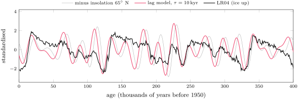
The lag model driven by the mid-July insolation at 65 N (less sunshine, more ice), against the benthic stack, all three standardised (mean 0, standard deviation 1); positive values mean more ice. The model follows the precession wiggles of the stack but has none of its large saw-tooth cycles. The response time of 10\, kyr is a model choice. — The lag model driven by the mid-July insolation at $65{}^{\circ}$ N (less sunshine, more ice), against the benthic stack, all three standardised (mean 0, standard deviation 1); positive values mean more ice. The model follows the precession wiggles of the stack but has none of its large saw-tooth cycles. The response time of $10\,\mathrm{kyr}$ is a model choice.

Over the last $800\,000$ years, the lagged model correlates with the stack at $r = 0.42$ , the insolation itself at only $0.23$ : the lag helps, but a linear ice sheet cannot make $100\,000$ -year cycles out of a forcing that has none. The terminations must involve non-linear behaviour that amplifies a modest push from the insolation. The candidates are feedbacks that act on the whole climate: the ice–albedo feedback of Definition 18.8, since a planet with more snow and ice reflects more sunlight; and carbon dioxide, which in the Antarctic ice cores rises on time scales of millennia whenever the overturning circulation of the Atlantic is weakened, as it is when meltwater from the ice sheets pours into the North Atlantic. Beyond a threshold of carbon dioxide, interglacial conditions can stabilise.

Definition 25.9 (Mid-Pleistocene transition)

The mid-Pleistocene transition is the change, from about $1\,250\,000$ to $700\,000$ years ago, from glacial cycles of about $41\,000$ years and small amplitude to quasi-periodic cycles of about $100\,000$ years and large amplitude, with thicker ice sheets, without any corresponding change in the orbital forcing.

Before the transition the ice sheets followed the obliquity, as the dashed spectrum of the figure above shows; one count finds a glacial termination in 67, 88 and $52\,\%$ of the obliquity cycles of the early, middle and late Quaternary. Orbital theory alone cannot explain the change; the candidates are the dynamics of the ice sheets themselves, perhaps after the removal of the soft regolith on which they slid, and a gradual decline of carbon dioxide during the glacial minima. No explanation is yet generally agreed.

25.5 Carbon dioxide in the glacial cycles

The Antarctic ice cores show that carbon dioxide follows the glacial cycles: between 188 and $194\,\mathrm{ppm}$ at the Last Glacial Maximum, between 266 and $282\,\mathrm{ppm}$ in the last interglacial; the composite record of Chapter 24 gives $189.7\,\mathrm{ppm}$ for 19 to $23\,\mathrm{ka}$ and $279.4\,\mathrm{ppm}$ over the two thousand years before industry. Its radiative forcing grows close to the logarithm of the concentration, $3.93\,\mathrm{W}\,\mathrm{m}^{-2}$ for each doubling.

Example 25.10 (Orbit against carbon dioxide)

From $189.7\,\mathrm{ppm}$ to $279.4\,\mathrm{ppm}$ , the forcing is $3.93\log_2(279.4/189.7) = 3.93 \times 0.559 = 2.2\,\mathrm{W}\,\mathrm{m}^{-2}$ , over the whole globe and the whole year. The orbit, over the last million years, changed the global and annual mean of the insolation by at most $340.54 - 340.00 = 0.54\,\mathrm{W}\,\mathrm{m}^{-2}$ , but the mid-July insolation at $65{}^{\circ}$ N by about $109\,\mathrm{W}\,\mathrm{m}^{-2}$ .

The orbit is a pacemaker, not an engine. It redistributes sunlight between seasons and latitudes and sets the timing; the ice sheets, by their albedo and their slowness, and carbon dioxide, by its global forcing, turn a regional signal into a global change of climate.

Exercises

Data for the exercises, unless stated otherwise: $S_0 = 1360\,\mathrm{W}\,\mathrm{m}^{-2}$ (the value of the tables); a tropical year of $365.2422$ days; the orbital elements of the tables, of which today $e = 0.017236$ , $\varpi = 101.37{}^{\circ}$ , $\varepsilon = 23.446{}^{\circ}$ .

Exercise 25.1 ★

Take $e = 0.0167$ . (a) Compute the ratio of the aphelion distance $a(1 + e)$ to the perihelion distance $a(1 - e)$ . (b) Express their difference as a percentage of $a$ . (c) By what factor is the sunlight at perihelion stronger than at aphelion?

Solution

Solution of Exercise 25.1.

(a) $1.0167/0.9833 = 1.0340$ : the aphelion is $3.4\,\%$ farther than the perihelion. (b) $a(1 + e) - a(1 - e) = 2ea = 0.0334\,a$ , $3.34\,\%$ of $a$ , close to the 3.4 per cent usually quoted. (c) Sunlight falls off as the inverse square of the distance: $1.0340^2 = 1.069$ , about $7\,\%$ more sunlight at perihelion.

Exercise 25.2 ★

The tables give $e = 0.017236$ , $\varpi = 101.37{}^{\circ}$ today; $e = 0.019971$ , $\varpi = 293.86{}^{\circ}$ $10\,000$ years ago; $e = 0.019249$ , $\varpi = 359.99{}^{\circ}$ $6000$ years ago. (a) Compute the climatic precession for each age. (b) For each, give the Sun’s longitude at perihelion. (c) At which age was the perihelion nearest the June solstice, and at which the September equinox?

Solution

Solution of Exercise 25.2.

(a) Today $0.017236 \times \sin101.37{}^{\circ} = 0.017236 \times 0.9804 = 0.01690$ ; $10\,000$ years ago $0.019971 \times \sin293.86{}^{\circ} = 0.019971 \times (-0.9145) = -0.01826$ ; $6000$ years ago $0.019249 \times \sin359.99{}^{\circ} \approx 0$ , the values of the tables. (b) The Sun’s longitude at perihelion is $\varpi + 180{}^{\circ}$ : $281.37{}^{\circ}$ today, $473.86{}^{\circ}$ $-$ $360{}^{\circ}$ $=$ $113.86{}^{\circ}$ $10\,000$ years ago, $179.99{}^{\circ}$ $6000$ years ago. (c) $10\,000$ years ago the perihelion fell $24{}^{\circ}$ after the June solstice, the nearest of the three to it, in the northern summer; $6000$ years ago it fell at the September equinox, where the climatic precession is zero.

Exercise 25.3 ★

The axis of rotation precesses with a period of about $25\,770$ years relative to the stars, while the orbit turns with a period of about $112\,000$ years. Assume that both motions move the perihelion relative to the equinox in the same sense, so that their frequencies add. (a) Combine the two frequencies to find the period with which the perihelion moves through the seasons. (b) Compare with the main periods of the climatic precession, $19.0$ , $22.4$ and $23.7$ thousand years.

Solution

Solution of Exercise 25.3.

(a) The frequencies add: $1/25.77 + 1/112 = 0.03880 + 0.00893 = 0.047\,73\,\mathrm{kyr}^{-1}$ , a period of $1/0.04773 = 21.0$ thousand years. (b) The result falls within the range of the main periods, 19.0 to 23.7 thousand years. A single number cannot reproduce them: the turning of the orbit is itself the sum of several motions with different frequencies, each of which combines with the precession of the axis to give one period of the climatic precession; the average is the $23\,000$ years usually quoted.

Exercise 25.4 ★

With Proposition 25.5 and $e = 0.0167$ , compute the annual-mean insolation at the North Pole for obliquities of $22.1{}^{\circ}$ and $24.5{}^{\circ}$ . By what percentage does it grow between the two?

Solution

Solution of Exercise 25.4.

$\sqrt{1 - 0.0167^2} = 0.99986$ . For $22.1{}^{\circ}$ : $1360 \times 0.37622/(\pi \times 0.99986) = 162.9\,\mathrm{W}\,\mathrm{m}^{-2}$ ; for $24.5{}^{\circ}$ : $1360 \times 0.41469/(\pi \times 0.99986) = 179.5\,\mathrm{W}\,\mathrm{m}^{-2}$ . The ratio is $\sin24.5{}^{\circ}/\sin22.1{}^{\circ} = 1.102$ : the annual mean at the pole grows by $10.2\,\%$ , about $16.7\,\mathrm{W}\,\mathrm{m}^{-2}$ , between the two extremes.

Exercise 25.5 ★★

(a) Compute exactly the distance factor $(a/r)^2$ at the June solstice today and $116\,000$ years ago ( $e = 0.043988$ , $\varpi = 92.71{}^{\circ}$ ), and compare with the approximation $1 - 2e\sin\varpi$ . (b) Compute both at the December solstice. (c) Why is the approximation worse $116\,000$ years ago?

Solution

Solution of Exercise 25.5.

(a) At the June solstice $(a/r)^2 = \bigl((1 - e\sin\varpi)/(1 - e^2)\bigr)^2$ . Today $e\sin\varpi = 0.016898$ and $(0.983102/0.999703)^2 = 0.9671$ , against $1 - 0.033796 = 0.9662$ ; $116\,000$ years ago $e\sin\varpi = 0.043939$ and $(0.956061/0.998065)^2 = 0.9176$ , against $1 - 0.087878 = 0.9121$ . (b) At the December solstice $(a/r)^2 = \bigl((1 + e\sin\varpi)/(1 - e^2)\bigr)^2$ : today $1.0347$ against $1.0338$ , $116\,000$ years ago $1.0940$ against $1.0879$ . (c) The neglected terms are of order $e^2$ : $(1 - x)^2/(1 - e^2)^2 \approx 1 - 2x + x^2 + 2e^2$ with $x = e\sin\varpi$ , here about $3e^2$ . They are $3 \times 0.0172^2 = 0.0009$ today and $3 \times 0.0440^2 = 0.0058$ $116\,000$ years ago, close to the differences found, $0.0009$ and $0.0055$ : the approximation is six times worse when the eccentricity is two and a half times larger.

Exercise 25.6 ★★

Reproduce Example 25.4 step by step: the hour angle of sunset at $65{}^{\circ}$ N at the June solstice, the length of the day, the insolation at the mean distance and the insolation of today.

Solution

Solution of Exercise 25.6.

At the June solstice $\delta = \varepsilon = 23.446{}^{\circ}$ . $\cos h_0 = -\tan65{}^{\circ}\tan23.446{}^{\circ} = -2.14451 \times 0.43369 = -0.93006$ , so $h_0 = 158.44{}^{\circ} = 2.7654\,\mathrm{rad}$ . The day lasts $2 \times 158.44/15 = 21.13$ hours (the Earth turns $15{}^{\circ}$ an hour). With $\sin65{}^{\circ} = 0.90631$ , $\cos65{}^{\circ} = 0.42262$ , $\sin\delta = 0.39788$ , $\cos\delta = 0.91744$ and $\sin h_0 = 0.36742$ , the bracket is $2.7654 \times 0.90631 \times 0.39788 + 0.42262 \times 0.91744 \times 0.36742 = 0.99720 + 0.14246 = 1.13966$ . At the mean distance $\bar Q = (1360/\pi) \times 1.13966 = 432.90 \times 1.13966 = 493.4\,\mathrm{W}\,\mathrm{m}^{-2}$ ; with the distance factor of Exercise 25.5, $493.4 \times 0.9671 = 477.1\,\mathrm{W}\,\mathrm{m}^{-2}$ . As a check, the same steps at $60{}^{\circ}$ N give $475.96\,\mathrm{W}\,\mathrm{m}^{-2}$ , where the tables give $475.95$ .

Exercise 25.7 ★★

(a) Using $\mathrm dt = T(r/a)^2\,\mathrm d\lambda/(2\pi\sqrt{1 - e^2})$ and $(r/a)^2 \approx 1 + 2e\cos(\lambda - \varpi)$ , show that the half-year from the March to the September equinox lasts about $T/2 + (2T/\pi)\,e\sin\varpi$ . (b) Compute by how many days it exceeds the other half-year today. (c) Compare with the 4.5 days by which northern summers exceed winters and the three days by which springs exceed autumns.

Solution

Solution of Exercise 25.7.

(a) The March equinox is $\lambda = 0$ , the September equinox $\lambda = \pi$ . With $\sqrt{1 - e^2} \approx 1$ , the duration is $\frac{T}{2\pi}\int_0^{\pi}\bigl(1 + 2e\cos(\lambda - \varpi)\bigr)\,\mathrm d\lambda = \frac{T}{2\pi}\bigl(\pi + 2e[\sin(\lambda - \varpi)]_0^{\pi}\bigr) = \frac{T}{2\pi}(\pi + 4e\sin\varpi) = \frac T2 + \frac{2T}{\pi}e\sin\varpi$ . (b) The other half-year is shorter by the same amount, so the difference is $(4T/\pi)\,e\sin\varpi = (4 \times 365.2422/\pi) \times 0.016898 = 465.04 \times 0.016898 = 7.86$ days. (c) Spring and summer together exceed autumn and winter by $4.5 + 3 = 7.5$ days; the two differences quoted are rounded, and the agreement is within that rounding.

Exercise 25.8 ★★

Over the last million years the eccentricity ranged from $0.0046$ to $0.0565$ . (a) Compute the global and annual mean insolation $S_0/(4\sqrt{1 - e^2})$ at both extremes. (b) By how much, in $\mathrm{W}\,\mathrm{m}^{-2}$ and in per cent, did the orbit change it? (c) Compare with the range of the mid-July insolation at $65{}^{\circ}$ N, 388 to $497\,\mathrm{W}\,\mathrm{m}^{-2}$ .

Solution

Solution of Exercise 25.8.

(a) For $e = 0.0046$ : $\sqrt{1 - e^2} = 0.999989$ and $340/0.999989 = 340.004\,\mathrm{W}\,\mathrm{m}^{-2}$ . For $e = 0.0565$ : $\sqrt{1 - 0.003192} = 0.998403$ and $340/0.998403 = 340.544\,\mathrm{W}\,\mathrm{m}^{-2}$ . (b) The difference is $0.54\,\mathrm{W}\,\mathrm{m}^{-2}$ , $0.16\,\%$ . (c) The mid-July insolation at $65{}^{\circ}$ N swung by $497 - 388 = 109\,\mathrm{W}\,\mathrm{m}^{-2}$ , about $25\,\%$ of its mean and two hundred times the change of the global annual mean: the orbit acts on climate by moving sunlight between seasons and latitudes, not by changing the total.

Exercise 25.9 ★★

With the lag model and $\tau = 10\,\mathrm{kyr}$ , compute the relative amplitude and the lag of the ice volume for sinusoidal forcing of periods 23, 41 and $100$ thousand years. Which band does the ice sheet favour, and why?

Solution

Solution of Exercise 25.9.

With $\omega = 2\pi/P$ and $\tau = 10\,\mathrm{kyr}$ : for $P = 23$ , $\omega\tau = 2.732$ , a relative amplitude $1/\sqrt{1 + 7.464} = 0.344$ and a lag $\arctan(2.732)/\omega = 1.2199/0.2732 = 4.47$ kyr; for $P = 41$ , $\omega\tau = 1.532$ , amplitude $0.546$ , lag $0.9926/0.1532 = 6.48$ kyr; for $P = 100$ , $\omega\tau = 0.628$ , amplitude $0.847$ , lag $0.5610/0.0628 = 8.93$ kyr. The ice sheet favours the slow forcing: it follows $85\,\%$ of a $100\,000$ -year cycle but only a third of a precession cycle, since it has too little time to grow or shrink before a fast forcing reverses. It acts as a low-pass filter.

Exercise 25.10 ★★★

The mid-July insolation at $65{}^{\circ}$ N has almost no power at $100\,000$ years, yet the ice volume of the last $700\,000$ years has most of its power there. (a) Show that if the forcing is $A_1\sin \omega_1 t + A_2\sin\omega_2 t$ , the lag model responds only at $\omega_1$ and $\omega_2$ . (b) Show that a response containing the term $V^2$ , for example $\mathrm dV/\mathrm dt = (V_{\mathrm{eq}} - V)/\tau + kV^2$ , can create the frequencies $\omega_1 - \omega_2$ and $\omega_1 + \omega_2$ , by substituting the linear solution into $V^2$ . (c) Two precession terms of periods $23.7$ and $19.0$ thousand years beat with what period? What do you conclude about the $100\,000$ -year cycles?

Solution

Solution of Exercise 25.10.

(a) The equation is linear: if $V_1$ answers $A_1\sin\omega_1t$ and $V_2$ answers $A_2\sin\omega_2t$ , $V_1 + V_2$ answers their sum. By Proposition 25.8 $V_1$ and $V_2$ are sinusoids of frequencies $\omega_1$ and $\omega_2$ (once the transient has died away), so the response holds no other frequency. (b) With $V \approx B_1\sin(\omega_1t - \phi_1) + B_2\sin(\omega_2t - \phi_2)$ ,

\begin{aligned} V^2 &= \tfrac12(B_1^2 + B_2^2) - \tfrac12B_1^2\cos(2\omega_1t - 2\phi_1) - \tfrac12B_2^2\cos(2\omega_2t - 2\phi_2)\\ &\quad + B_1B_2\bigl[\cos\bigl((\omega_1 - \omega_2)t - \phi_1 + \phi_2\bigr) - \cos\bigl((\omega_1 + \omega_2)t - \phi_1 - \phi_2\bigr)\bigr], \end{aligned}

so the term $kV^2$ forces the equation at the difference and sum frequencies, and at the double frequencies. (c) $1/(1/19.0 - 1/23.7) = 1/(0.05263 - 0.04219) = 95.8$ thousand years; the pair 19.0 and 22.4 gives 125 thousand years. The difference frequencies of the precession terms fall in the eccentricity band, as they must, since the climatic precession is $e\sin\varpi$ . A non-linear ice sheet could therefore draw a $100\,000$ -year rhythm out of the precession; a linear one cannot. The $100\,000$ -year cycles are evidence of non-linear behaviour, though this calculation alone does not show which.

Exercise 25.11 ★★★

At the North Pole, the energy received per square metre during the polar day is $E = \int S_0(a/r)^2 \sin\delta\,\mathrm dt$ over the half-year when $\delta > 0$ . (a) Show with the proof of Proposition 25.5 that $E = S_0T\sin\varepsilon/(\pi\sqrt{1 - e^2})$ . (b) Compute $E$ in $\mathrm{GJ}\,\mathrm{m}^{-2}$ for $\varepsilon = 22.1{}^{\circ}$ and $24.5{}^{\circ}$ , with $e = 0.0167$ and $T$ = 365.25 days. (c) The precession does not appear in $E$ . Why can it nevertheless change the melting of an ice sheet?

Solution

Solution of Exercise 25.11.

(a) As in the proof of Proposition 25.5, $(a/r)^2\,\mathrm dt = T\,\mathrm d\lambda/(2\pi\sqrt{1 - e^2})$ , and $\sin\delta = \sin\varepsilon\sin\lambda$ is positive for $0 < \lambda < \pi$ . So $E = \frac{S_0T\sin\varepsilon}{2\pi\sqrt{1 - e^2}}\int_0^{\pi}\sin\lambda \,\mathrm d\lambda = S_0T\sin\varepsilon/(\pi\sqrt{1 - e^2})$ . (b) $T = 365.25 \times 86400 = 3.1558 \times 10^{7}\,\mathrm{s}$ , $S_0T/\pi = 1.3661 \times 10^{10}\,\mathrm{J}\,\mathrm{m}^{-2}$ ; for $22.1{}^{\circ}$ , $E = 1.3661 \times 10^{10} \times 0.37622/0.99986 = 5.14\,\mathrm{GJ}\,\mathrm{m}^{-2}$ ; for $24.5{}^{\circ}$ , $5.67\,\mathrm{GJ}\,\mathrm{m}^{-2}$ , $10\,\%$ more. (c) The precession fixes how the same energy is spread in time: a summer at perihelion is shorter and more intense, a summer at aphelion longer and weaker. Melting starts only above $0\,{}^{\circ}\mathrm{C}$ , so a short intense summer can melt more than a long cool one receiving the same total.

Exercise 25.12 ★★★

(a) Compute the radiative forcing of the rise of carbon dioxide from $189.7\,\mathrm{ppm}$ to $279.4\,\mathrm{ppm}$ , with $3.93\,\mathrm{W}\,\mathrm{m}^{-2}$ per doubling and a logarithmic law. (b) The ranges given for the Last Glacial Maximum and the last interglacial are 188 to $194\,\mathrm{ppm}$ and 266 to $282\,\mathrm{ppm}$ : compute the smallest and the largest forcing they allow. (c) Compare with the change of the global annual insolation of Exercise 25.8 and with the swing of the $65{}^{\circ}$ N summer insolation. Which is the trigger and which the amplifier?

Solution

Solution of Exercise 25.12.

(a) $3.93\log_2(279.4/189.7) = 3.93\log_2 1.4729 = 3.93 \times 0.5586 = 2.20\,\mathrm{W}\,\mathrm{m}^{-2}$ . (b) The smallest rise is from 194 to $266\,\mathrm{ppm}$ : $3.93\log_2 1.3711 = 3.93 \times 0.4554 = 1.79\,\mathrm{W}\,\mathrm{m}^{-2}$ ; the largest from 188 to $282\,\mathrm{ppm}$ : $3.93\log_2 1.5 = 3.93 \times 0.5850 = 2.30\,\mathrm{W}\,\mathrm{m}^{-2}$ . (c) The forcing of carbon dioxide is four times the largest change of the global annual insolation, $0.54\,\mathrm{W}\,\mathrm{m}^{-2}$ , and it acts everywhere and all year; the summer insolation at $65{}^{\circ}$ N swings by about $109\,\mathrm{W}\,\mathrm{m}^{-2}$ , but at one latitude and one season. The orbit is the trigger, through the summers of the northern ice sheets; carbon dioxide, with the ice–albedo feedback, is an amplifier that spreads the change over the globe.

Problem 25.1

Weekend problem — Sunlight at $65{}^{\circ}$ N

The last interglacial ended about $116\,000$ years ago. How much sunshine did the summer of the latitude of the great northern ice sheets receive then, compared with today? Use the data of the exercises. The tables give, $116\,000$ years ago, $e = 0.0440$ , $\varpi = 92.7{}^{\circ}$ , $\varepsilon = 22.52{}^{\circ}$ ; today, rounded in the same way, $e = 0.0172$ , $\varpi = 101.4{}^{\circ}$ , $\varepsilon = 23.45{}^{\circ}$ .

Part I — The orbit then and now.

Compute the climatic precession then and now.
Compute the perihelion and aphelion distances, in units of $a$ , then and now.
At what longitude of the Sun was the Earth at perihelion then, and now? Near which solstice?
By what factor was the sunlight at perihelion stronger than at aphelion, then and now?
Was the obliquity larger or smaller than today? What does that mean for the summers of the high latitudes?
Compute the global and annual mean insolation then and now. Is the difference significant?

Part II — The distance at the June solstice.

Show from Proposition 25.3 that at the June solstice $r/a = (1 - e^2)/(1 - e\sin\varpi)$ .
Compute $r/a$ at the June solstice then and now.
Compute $(a/r)^2$ then and now.
Compare with the approximation $1 - 2e\sin\varpi$ .
By what percentage was the solstice sunlight weaker than at the mean distance, then and now?

Part III — Sunshine at $65{}^{\circ}$ N.

Give the declination of the Sun at the June solstice then and now.
Compute the hour angle of sunset at $65{}^{\circ}$ N on that day, then and now.
Deduce the length of the day.
Compute the daily-mean insolation at the mean distance.
Compute the daily-mean insolation, then and now.
The tables give, for mid-July, 397.60 and $426.76\,\mathrm{W}\,\mathrm{m}^{-2}$ . Why are the solstice values higher?
Which counted more in the difference between then and now, the obliquity or the distance?

Part IV — The ice sheet’s answer.

In the lag model with $\tau = 10\,\mathrm{kyr}$ , what fraction of a sudden change of $V_{\mathrm{eq}}$ has the ice sheet achieved after 5, 10 and $20\,\mathrm{kyr}$ ?
The June insolation at $65{}^{\circ}$ N fell from a maximum about $128\,000$ years ago to the minimum of $116\,000$ years ago, half a precession cycle. For a sinusoid of period $23\,\mathrm{kyr}$ , what fraction of the forcing does the ice sheet follow, and how late?
Why can an ice sheet not reach, within one precession cycle, the size that a low summer insolation would sustain?
The ice took some $90\,000$ years to build up to the Last Glacial Maximum and about $10\,000$ years to melt. Why can the lag model not produce that asymmetry?
Carbon dioxide stood between 266 and $282\,\mathrm{ppm}$ in the last interglacial and between 188 and $194\,\mathrm{ppm}$ at the Last Glacial Maximum. How does it help a regional change of sunshine become a global change of climate?
To sum up: what was the daily-mean insolation at $65{}^{\circ}$ N on the June solstice when the last interglacial ended, $116\,000$ years ago?

Solution

Solution of Problem 25.1.

1. Then $0.0440 \times \sin92.7{}^{\circ} = 0.0440 \times 0.99889 = 0.04395$ ; now $0.0172 \times \sin101.4{}^{\circ} = 0.0172 \times 0.98027 = 0.01686$ , about 2.6 times less. 2. Then $1 - 0.0440 = 0.956$ and $1 + 0.0440 = 1.044$ ; now $0.9828$ and $1.0172$ . 3. At $\lambda = \varpi + 180{}^{\circ}$ : then $272.7{}^{\circ}$ , now $281.4{}^{\circ}$ , both near the December solstice ( $\lambda = 270{}^{\circ}$ ); then the Earth passed perihelion less than three days after it, and aphelion at the June solstice. 4. Then $(1.044/0.956)^2 = 1.0921^2 = 1.193$ , now $(1.0172/0.9828)^2 = 1.0350^2 = 1.071$ : $19\,\%$ more sunlight at perihelion then, $7\,\%$ now. 5. Smaller, $22.52{}^{\circ}$ against $23.45{}^{\circ}$ : the summer sun stood lower at high latitudes, and high latitudes received less sunlight in summer and over the year. 6. Then $340/\sqrt{1 - 0.001936} = 340/0.999032 = 340.33\,\mathrm{W}\,\mathrm{m}^{-2}$ ; now $340/0.999852 = 340.05\,\mathrm{W}\,\mathrm{m}^{-2}$ . The difference, $0.28\,\mathrm{W}\,\mathrm{m}^{-2}$ or less than one part in a thousand, is insignificant. 7. At $\lambda = 90{}^{\circ}$ , $\cos(90{}^{\circ} - \varpi) = \sin\varpi$ in Proposition 25.3. 8. Then $(1 - 0.001936)/(1 - 0.04395) = 0.998064/0.956049 = 1.04395$ ; now $(1 - 0.000296)/(1 - 0.01686) = 0.999704/0.983139 = 1.01685$ . 9. Then $1/1.04395^2 = 0.91758$ ; now $1/1.01685^2 = 0.96714$ . 10. Then $1 - 2 \times 0.04395 = 0.91210$ ; now $1 - 2 \times 0.01686 = 0.96628$ : the approximation errs by $0.0055$ then, $0.0009$ now. 11. Then $1 - 0.91758 = 8.2\,\%$ weaker, now $3.3\,\%$ . 12. At the solstice $\delta = \varepsilon$ : $22.52{}^{\circ}$ then, $23.45{}^{\circ}$ now. 13. Then $\cos h_0 = -2.14451 \times 0.41462 = -0.88916$ , $h_0 = 152.77{}^{\circ} = 2.6663\,\mathrm{rad}$ ; now $\cos h_0 = -2.14451 \times 0.43378 = -0.93023$ , $h_0 = 158.47{}^{\circ} = 2.7659\,\mathrm{rad}$ . 14. $2h_0/15{}^{\circ}$ per hour: then $20.37$ hours, now $21.13$ hours. 15. Then $2.6663 \times 0.90631 \times 0.38301 + 0.42262 \times 0.92375 \times 0.45759 = 0.92554 + 0.17864 = 1.10418$ ( $1.104\,17$ unrounded), and $432.90 \times 1.10417 = 478.0\,\mathrm{W}\,\mathrm{m}^{-2}$ ; now $2.7659 \times 0.90631 \times 0.39795 + 0.42262 \times 0.91741 \times 0.36697 = 0.99757 + 0.14228 = 1.13985$ ( $1.139\,82$ unrounded), and $432.90 \times 1.13982 = 493.4\,\mathrm{W}\,\mathrm{m}^{-2}$ . 16. Then $478.0 \times 0.91758 = 438.6\,\mathrm{W}\,\mathrm{m}^{-2}$ ; now $493.4 \times 0.96714 = 477.2\,\mathrm{W}\,\mathrm{m}^{-2}$ , $38.6\,\mathrm{W}\,\mathrm{m}^{-2}$ more than then. 17. In mid-July the Sun’s longitude is $120{}^{\circ}$ : $\sin\delta = \sin\varepsilon\sin120{}^{\circ}$ , a declination of about $20{}^{\circ}$ instead of $23{}^{\circ}$ , so a shorter day and a lower sun: at $65{}^{\circ}$ N the daily-mean insolation is greatest near the solstice, when the declination is largest. 18. With today’s distance, the change of obliquity alone costs $(493.4 - 478.0) \times 0.96714 = 14.9\,\mathrm{W}\,\mathrm{m}^{-2}$ ; with the old obliquity, the distance alone costs $478.0 \times (0.96714 - 0.91758) = 23.7\,\mathrm{W}\,\mathrm{m}^{-2}$ . The two add to $38.6\,\mathrm{W}\,\mathrm{m}^{-2}$ ; the distance counted for about three fifths. 19. After a sudden change the ice sheet has achieved $1 - \mathrm e^{-t/\tau}$ of it: $1 - \mathrm e^{-0.5} = 0.39$ after $5\,\mathrm{kyr}$ , $1 - \mathrm e^{-1} = 0.63$ after $10\,\mathrm{kyr}$ , $1 - \mathrm e^{-2} = 0.86$ after $20\,\mathrm{kyr}$ . 20. $\omega\tau = 2\pi \times 10/23 = 2.732$ : the ice sheet follows $1/\sqrt{1 + 2.732^2} = 0.34$ of the forcing, $\arctan(2.732)/\omega = 4.5$ kyr late. 21. Half a precession cycle, some 11 to $12\,\mathrm{kyr}$ , is about one response time: before the ice sheet has covered two thirds of the way, the insolation turns round and pulls it back. 22. In the linear model the ice grows and shrinks at the same rate for forcings of the same size: a rising and a falling forcing give mirror-image responses. A slow build-up followed by a fast collapse needs a response that depends on the state or the direction of change, that is a non-linear one. 23. Carbon dioxide rose by $3.93\log_2(266/194) = 1.8$ to $3.93\log_2(282/188) = 2.3\,\mathrm{W}\,\mathrm{m}^{-2}$ from glacial to interglacial: a forcing over the whole globe and the whole year. Released when the Atlantic circulation weakens, it carries the change of the northern summers to the whole planet, and, with the albedo of the shrinking ice, amplifies it. 24. When the last interglacial ended, the June-solstice daily-mean insolation at $65{}^{\circ}$ N was about $439\,\mathrm{W}\,\mathrm{m}^{-2}$ , $39\,\mathrm{W}\,\mathrm{m}^{-2}$ less than today and its lowest value of the cycle.

本章定义的术语

在术语表中查看全部 957 个术语