26Climate over Geological Time

Fifty million years ago no ice sheet stood anywhere on the Earth. The air held more than a thousand parts per million of carbon dioxide, the poles had warmed far more than the equator, and forests of a nearly tropical kind grew at $70{}^{\circ}$ S, through the months of polar night. Thirty-four million years ago ice spread over Antarctica, and it has never left. Over the hundreds of millions of years recorded in the rocks, the Earth has swung between such worlds, with ice and without; yet it has never boiled its oceans away nor frozen for good since the snowballs of Chapter 18. This chapter follows the carbon that sets these climates, the slow cycle that moves it between the air and the rocks, and the thermostat that keeps the planet habitable.

You already know

From the school volumes: the greenhouse effect and radiative forcing; the forcing of carbon dioxide grows with the logarithm of its concentration, $3.93\,\mathrm{W}\,\mathrm{m}^{-2}$ for a doubling; equilibrium climate sensitivity, best estimate $3\,{}^{\circ}\mathrm{C}$; outgassing; the glacial cycles and the Last Glacial Maximum. From the Year 1 volume: chemical weathering and the hydrolysis of silicates; clay minerals; carbonate oozes, the lysocline and the carbonate compensation depth. From earlier chapters: the faint young Sun and snowball Earth (Chapter 18); palaeogeography and oceanic anoxic events (Chapter 19); climate proxies, $\delta^{18}$O and the ice-volume effect (Chapter 24); orbital forcing (Chapter 25). The carbon cycle, its reservoirs and the residence time belong to the biology books, the Arrhenius law to the chemistry books.

26.1 The long-term carbon cycle

Reservoirs and fluxes

Definition 26.1 (Long-term carbon cycle; carbonate–silicate cycle)

The long-term carbon cycle is the exchange of carbon between the surface reservoirs (atmosphere, ocean, biosphere and soils) and the solid Earth: volcanic and metamorphic degassing, the weathering of rocks, and the burial of carbonate and organic carbon in sediments that later become rock or are subducted. Its fluxes are small against the surface reservoirs and act over $10^5$ to $10^8$ years. The carbonate–silicate cycle is its inorganic part: carbon dioxide leaves the mantle and the crust at volcanoes, is consumed by the weathering of silicate rocks, is deposited on the sea floor as carbonate, and returns to the surface when that carbonate is metamorphosed or subducted and degassed.

The biology books follow carbon through photosynthesis, respiration and the ocean over years to centuries. On the time scale of climate history the picture widens to include the rocks. Before the industrial era the atmosphere held $591\,\mathrm{PgC}$ (petagrams, or billions of tonnes, of carbon); the ocean held $38\,700$, nearly all of it as dissolved inorganic carbon in the intermediate and deep water ($37\,100$); vegetation, soils and permafrost held $3350$ between them. The active surface reservoirs together hold about $3.5 \times 10^{6}$ teramoles of carbon, some $42\,000\,\mathrm{PgC}$. The sedimentary rocks hold carbon too, as limestone and as organic matter scattered through shales, and they exchange it with the surface only slowly.

A modern estimate of the inputs and outputs, in teramoles of carbon a year ($1\,\mathrm{Tmol}$ of carbon is $0.012\,\mathrm{PgC}$), runs as follows. Into the ocean and atmosphere: volcanic degassing at mid-ocean ridges (1.3), ocean islands (1.3), arcs (4.5) and continental rifts (4.2), about 11 in all; metamorphic degassing, 2 to 4; the weathering of old carbonate, 12.3, and the oxidation of old organic carbon exposed by erosion, 8.1, with 2.0 from geological methane: $36.7$ in all. Out of them: carbonate sedimentation, about 26, and the burial of organic carbon, about 16. The two sides balance within their uncertainties. Degassing from the Earth’s interior supplies little more than a third of the input (Exercise 26.2); the rest is old sedimentary carbon on its way round again. Other estimates of the volcanic flux are lower, $0.1\,\mathrm{PgC}$ a year (about 8 Tmol) in the global carbon budget of the IPCC, or $0.26\,\mathrm{Gt}$ of carbon dioxide (about 6 Tmol of carbon) in a survey of the US Geological Survey: the volcanic input is known to within a factor of two.

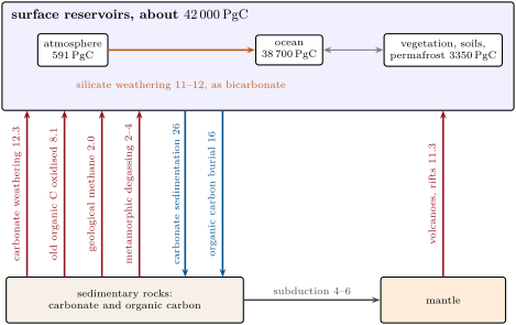
Divided by the flux through them, the $3.5 \times 10^{6}\,\mathrm{Tmol}$ of the surface reservoirs give a residence time of carbon of 8 to $9 \times 10^{4}$ years. Carbon that enters the ocean and air is buried again within some hundred thousand years, a blink on the scale of this chapter: the surface reservoirs follow the slow inputs and outputs closely, and any lasting imbalance between them changes the carbon dioxide of the air.

Carbonate and silicate weathering

Rain dissolves carbon dioxide and attacks rocks, as the Year 1 volume described. Two kinds of rock behave very differently. Weathering a limestone takes one carbon dioxide from the air and one carbon from the rock into the water; when a marine organism builds its shell from the products, one carbon goes back to the air:

The round trip is null for the air. Weathering a silicate, written here with wollastonite as a stand-in for the calcium silicates of granite and basalt, also takes carbon dioxide, but brings none from the rock:

and the carbonate built from it sends back only one of the two:

Each mole of calcium or magnesium silicate weathered on land thus locks one mole of carbon dioxide into carbonate rock. This is why carbonate sedimentation, about 26, exceeds carbonate weathering, 12.3, by roughly the 11 to 12 teramoles a year that silicate weathering consumes; and it is the silicate weathering, not the carbonate, that balances the volcanoes over millions of years.

26.2 The silicate-weathering thermostat

A negative feedback

Silicate weathering is a chemical reaction, and like most it is faster when it is warm. Warmth also brings more rain and more run-off, which carry the products away and bring fresh water to the rock. The rate therefore rises with temperature; and temperature rises with the carbon dioxide of the air. A planet that gains carbon dioxide warms, weathers faster and loses it again.

Definition 26.2 (Silicate-weathering thermostat)

The silicate-weathering thermostat is the negative feedback between climate and the long-term carbon cycle: the weathering of silicate rocks, which removes carbon dioxide from the atmosphere into carbonate rock, increases with temperature and run-off, so that a rise of atmospheric carbon dioxide raises the rate of its own removal and a fall lowers it. Over $10^5$ to $10^6$ years it brings the removal back into balance with the degassing.

The temperature dependence is that of the Arrhenius law of the chemistry books. With an activation energy $E_{\text a}$ for the dissolution of calcium and magnesium silicates, the weathering flux at a temperature $T$ near a reference $T_0$ is

since $1/T - 1/T_0 \approx -(T - T_0)/T_0^2$. Laboratory dissolution gives $E_{\text a} = 63\,\mathrm{kJ}\,\mathrm{mol}^{-1}$, and with $T_0 = 288\,\mathrm{K}$, $k_T = 0.09\,\mathrm{K}^{-1}$: the flux grows by about $9\,\%$ for each degree; within ten degrees of $T_0$ the approximation departs from the exact law by less than $3\,\%$ (Exercise 26.6). A field estimate is $74 \pm 29\,\mathrm{kJ}\,\mathrm{mol}^{-1}$, so the sensitivity is uncertain by a factor of about two. Run-off adds to it: with a flux proportional to $(R/R_0)^{0.65}$ and a run-off that rises by $4.5\,\%$ per degree, the combined sensitivity becomes $k = 0.09 + 0.65\times0.045 = 0.119\,\mathrm{K}^{-1}$.

A one-box model

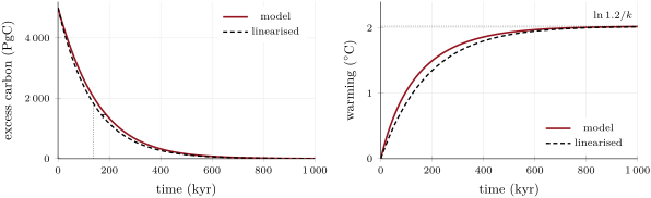
To see how fast the thermostat works, follow the excess carbon $M$ that the ocean and atmosphere hold above a steady state. Within a few thousand years of a disturbance the ocean and the sea-floor carbonates have taken most of an excess out of the air; for a release of $4000\,\mathrm{PgC}$, about $8\,\%$ stays in the air until silicate weathering removes it. Write $f$ for that fraction and $A_0 = 591\,\mathrm{PgC}$ for the air’s pre-industrial carbon, so that the carbon dioxide of the air is $C = C_0(1 + fM/A_0)$. The warming follows the logarithmic law with the climate sensitivity $S$, $\Delta T = S\log_2(C/C_0)$, and the weathering follows the exponential law above.

Proposition 26.3 (The thermostat’s steady state and time constant)

Let the excess carbon $M$ of the ocean–atmosphere change as

$$\frac{\mathrm dM}{\mathrm dt} = V - W_0\,e^{k\,\Delta T(M)}, \qquad \Delta T(M) = S\log_2\Bigl(1 + \frac{fM}{A_0}\Bigr),$$

where $V$ is the degassing and $W_0$ the weathering at $M = 0$.

1. The steady state has $\Delta T^* = \ln(V/W_0)/k$, whatever $S$ and $f$.

2. If $V = W_0$, a small excess decays as $M(t) = M(0)\,e^{-t/\tau}$ with

   $$\tau = \frac{A_0 \ln 2}{f\,k\,S\,W_0} .$$

The first result is the heart of the thermostat. It fixes a temperature, not a concentration: if the volcanoes degas $20\,\%$ more, the Earth settles $\ln 1.2/0.09 = 2.0\,{}^{\circ}\mathrm{C}$ warmer, whatever its climate sensitivity, and the carbon dioxide adjusts to whatever gives that warming, here $60\,\%$ more. A weak weathering response, a small $k$, makes a poor thermostat; a strong one holds the temperature nearly fixed.

Example 26.4 (The thermostat’s time constant)

Silicate weathering consumes 11 to $12\,\mathrm{Tmol}$ of carbon a year; take $W_0 = 11.5\times0.012011 = 0.138\,\mathrm{PgC}\,\mathrm{yr}^{-1}$. With $A_0 = 591\,\mathrm{PgC}$, $f = 0.08$, $k = 0.09\,\mathrm{K}^{-1}$ and $S = 3\,\mathrm{K}$,

$$\tau = \frac{591\times0.693}{0.08\times0.09\times3\times0.138} = 1.37 \times 10^{5}\,\mathrm{yr} ,$$

about 140 thousand years. With the run-off factor, $k = 0.119$, it shortens to $104\,\mathrm{kyr}$.

The model is crude: the fraction $f$ is not a constant, the ocean’s chemistry is reduced to one number and the weathering to one global law. Models with an explicit ocean and sediment give e-folding times from about $200\,\mathrm{kyr}$ to a million years. The thermostat is therefore a regulator of the very long term: it does nothing to the climate of the next few thousand years, and it holds the Earth’s temperature within bounds over hundreds of millions.

The thermostat also explains the faint young Sun of Chapter 18. The Sun brightens by a few per cent every few hundred million years, and an Earth with fixed air would warm with it; but warmer means faster weathering, which draws the carbon dioxide down until the temperature returns close to where the degassing puts it. The rocks of the last 420 million years show exactly this, as the next section reads.

26.3 Greenhouse and icehouse worlds

Definition 26.5 (Greenhouse and icehouse climate states)

A greenhouse climate state is a long interval, millions to tens of millions of years, without large continental ice sheets, with high atmospheric carbon dioxide and a small temperature difference between the equator and the poles. An icehouse climate state is a long interval with continental ice sheets at one or both poles, lower carbon dioxide and a steep equator-to-pole gradient. The Earth has been in an icehouse state since about $34\,\mathrm{Ma}$.

Carbon dioxide over 420 million years

Carbon dioxide before the ice cores is read from proxies: the boron isotopes and organic molecules of marine plankton, the pores of fossil leaves, the carbonate nodules of ancient soils. A 2017 compilation of them back to $420\,\mathrm{Ma}$, smoothed, is shown below with the glaciations. Its long-term trend is a decline of about $3.4\,\mathrm{ppm}$ per million years, and values close to the pre-industrial level appear twice before our own time: in the Carboniferous and Permian, and briefly in the late Cretaceous.

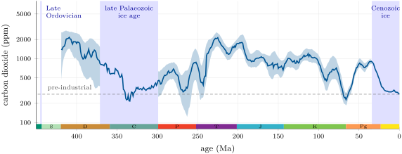
Over the same 420 million years the Sun brightened by about $4\,\%$, some $50\,\mathrm{W}\,\mathrm{m}^{-2}$ at the Earth’s distance and $9\,\mathrm{W}\,\mathrm{m}^{-2}$ of forcing once spread over the sphere and corrected for the albedo. The fall of carbon dioxide from about $1400\,\mathrm{ppm}$ to the pre-industrial value almost exactly cancels it (Exercise 26.7): in terms of forcing the Earth has stayed within a few watts per square metre of today for 420 million years, and its icehouse states came when the combined forcing of carbon dioxide and Sun fell below about 1 to $2\,\mathrm{W}\,\mathrm{m}^{-2}$. The authors of the compilation attribute the compensation to the silicate weathering feedback and the spread of land plants, whose roots and soils speed weathering.

Palaeozoic ice ages

A reconstruction of global mean surface temperature published in 2024, which combines proxy data with climate models, puts the Phanerozoic range between $11\,{}^{\circ}\mathrm{C}$, in the glacial times of the late Pleistocene, 129 to 11.7 thousand years ago, and $36\,{}^{\circ}\mathrm{C}$, in the Turonian, 94 to $89\,\mathrm{Ma}$ ago. Its warm and cold intervals follow the glaciations recorded by tillites and striated pavements.

The Late Ordovician glaciation, in the Hirnantian stage (445.2 to $443.1\,\mathrm{Ma}$), spread ice sheets over Gondwana, much of which lay near the South Pole (Chapter 19), and coincided with one of the five great extinctions. Its global mean temperature, about $21\,{}^{\circ}\mathrm{C}$ in the reconstruction, is warmer than that of later glaciations: the vast supercontinent made its interior cold enough for ice sheets anyway. The late Palaeozoic ice age is the longest of the Phanerozoic: its first glacial deposits are latest Devonian, its coldest global temperatures in the Serpukhovian, about 330 to $323\,\mathrm{Ma}$, and its greatest extent of ice towards the end of the Carboniferous, 307 to $299\,\mathrm{Ma}$. It coincides with the low carbon dioxide of the Carboniferous and Permian, which the compilation’s authors link to a weaker volcanic flux or stronger weathering while Pangaea was assembled and its mountains stood high.

The Cretaceous greenhouse

The warmest time of the reconstruction is the middle Cretaceous, the time of the high seas and the oceanic anoxic events of Chapter 19. The carbon dioxide estimates for it are puzzling: the compilation above gives some 450 to $860\,\mathrm{ppm}$ between 100 and $90\,\mathrm{Ma}$, and the 2024 reconstruction finds a median of about $775\,\mathrm{ppm}$ for its hottest intervals, lower than its temperatures suggest. Whether carbon dioxide and temperature truly parted company then, or the proxies misread the Cretaceous air, is open; the authors call it the “Mesozoic conundrum”.

26.4 The Cenozoic: from hothouse to icehouse

The best record of the last 66 million years is in the shells of benthic foraminifera, cored from the deep-sea floor. Their $\delta^{18}$O rises when the deep water cools and when ice sheets store the light isotope on land (Chapter 24). The figure below shows the reference record built in 2020 from deep-sea drill cores, averaged over $100\,\mathrm{kyr}$.

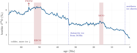
Read from right to left, the record tells four chapters. The early Cenozoic warmed, through the Palaeocene–Eocene Thermal Maximum, to the Early Eocene Climatic Optimum, 53 to $49\,\mathrm{Ma}$, when global temperature stood 10 to $18\,{}^{\circ}\mathrm{C}$ above that of 1850–1900 (medium confidence, in the language of the IPCC) and carbon dioxide between 1150 and $2500\,\mathrm{ppm}$. A long cooling followed, punctuated at the Eocene–Oligocene transition, about $34\,\mathrm{Ma}$, by a jump of about $1.5\,\text{‰}$ in $\delta^{18}$O: the first large ice sheet on Antarctica, with a deep-ocean cooling of the order of $2\,{}^{\circ}\mathrm{C}$. The Miocene Climatic Optimum, 16.9 to $14.7\,\mathrm{Ma}$, brought warmth back, 4 to $10\,{}^{\circ}\mathrm{C}$ above 1850–1900 with 400 to $600\,\mathrm{ppm}$. After the mid-Pliocene, the last time carbon dioxide stood near today’s 360 to $420\,\mathrm{ppm}$, it fell by some $30\,\mathrm{ppm}$ per million years, and from $2.7\,\mathrm{Ma}$ ice sheets grew durably in the northern hemisphere: the glacial cycles of Chapter 25 began.

Over the whole of the last 50 million years carbon dioxide fell at about $16\,\mathrm{ppm}$ per million years. The IPCC calls the cause uncertain, possibly an imbalance between volcanic degassing and the two long-term sinks, organic carbon burial and silicate weathering. A threshold of 750 to $1000\,\mathrm{ppm}$ has been modelled for the growth of permanent ice sheets on Antarctica; the last time carbon dioxide stood as high as $1000\,\mathrm{ppm}$ was just before the transition.

Figures as of 2023

In 2023 a consortium of researchers published a vetted compilation of all the Cenozoic carbon dioxide estimates then published. In its reconstruction carbon dioxide peaked near $1600\,\mathrm{ppm}$ around $51\,\mathrm{Ma}$; the onset of the Antarctic ice sheet, near $33.9\,\mathrm{Ma}$, came at $720\,\mathrm{ppm}$; by $32\,\mathrm{Ma}$ it had fallen to $550\,\mathrm{ppm}$; the Middle Miocene, about $16\,\mathrm{Ma}$, was the last time it stayed higher than today; and it fell below $270\,\mathrm{ppm}$ at $2.6\,\mathrm{Ma}$, when the Earth entered its present state of ice at both poles. Read against temperature, the curve gives an Earth system sensitivity — the warming per doubling once ice sheets and vegetation have responded — of about $8\,{}^{\circ}\mathrm{C}$ through the cooling to $34\,\mathrm{Ma}$, or $5\,{}^{\circ}\mathrm{C}$ with another temperature record: more than the $3\,{}^{\circ}\mathrm{C}$ of the fast feedbacks.

Tectonics and climate

Why did carbon dioxide fall? Two families of explanation draw on plate tectonics, and the IPCC’s summary names both: the drift of the plates built mountains, drove erosion and volcanism and reconfigured the ocean passages, and so moved carbon from the atmosphere into other reservoirs.

The first is weathering. Mountains weather faster than lowlands: steep slopes are scoured of their soil, and fresh rock is exposed to rain. The uplift of the Himalaya and the Tibetan Plateau since the India–Asia collision of Chapter 14 has been proposed to have raised global silicate weathering and drawn the carbon dioxide down. The thermostat makes this subtle: if the Earth’s “weatherability”, the factor $W_0$, rises at a fixed degassing, the steady temperature falls by $\ln(W_0'/W_0)/k$ (Exercise 26.9), but the thermostat still holds the removal equal to the degassing. Uplift changes the climate at which the balance is struck, not the balance itself. The hypothesis remains debated.

Definition 26.6 (Ocean gateway)

An ocean gateway is a strait or passage between two oceans whose opening, closing or deepening by plate motion changes the exchange of water, heat and salt between them, and so the ocean circulation.

The second is the ocean gateways, above all the Drake Passage between South America and Antarctica and the Tasman Gateway between Australia and Antarctica. Once both were deep, a current could flow right round Antarctica. The Tasman Gateway deepened beyond about $500\,\mathrm{m}$ at $33.5 \pm 1.5\,\mathrm{Ma}$, close to the transition; the Drake Passage opened earlier, perhaps by $50\,\mathrm{Ma}$, but shallow and narrow, and ridges may have blocked deep flow through it until about $22\,\mathrm{Ma}$. Models with the geography of the Eocene find that opening the gateways changes the heat carried towards Antarctica only modestly; the review of 2021 concludes that a fall of carbon dioxide, of perhaps $40\,\%$, best explains the transition, with the gateways and the ice sheet itself in a secondary role.

26.5 Hyperthermals and the PETM

The slow decline of carbon dioxide is interrupted by a few sudden spikes.

Definition 26.7 (Hyperthermal event; Palaeocene–Eocene Thermal Maximum)

A hyperthermal event is a geologically brief global warming, a few thousand to a few hundred thousand years long, caused by a rapid release of carbon to the ocean and atmosphere and recorded by a fall of the $\delta^{13}$C of marine and terrestrial carbon, a dissolution of sea-floor carbonate and a fall of $\delta^{18}$O. The Palaeocene–Eocene Thermal Maximum (PETM), 55.9 to $55.7\,\mathrm{Ma}$, is the largest of the Cenozoic; its onset marks the base of the Eocene.

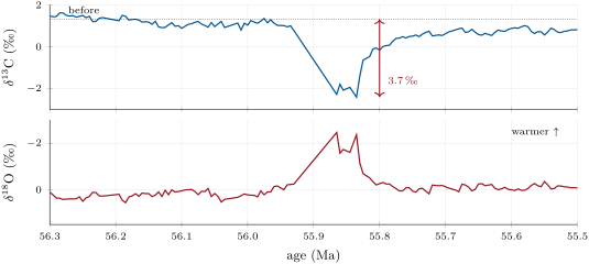
The IPCC’s assessment of the PETM runs as follows. Carbon dioxide rose from about 900 to more than $2000\,\mathrm{ppm}$; the carbon was released in 3 to $20\,\mathrm{kyr}$, between about 3000 and more than $7000\,\mathrm{PgC}$ of it (low to medium confidence), from methane hydrates, volcanoes, organic carbon on land and at sea, or a combination. The Earth warmed by 4 to $8\,{}^{\circ}\mathrm{C}$ above pre-industrial, about $5\,{}^{\circ}\mathrm{C}$ above the climate just before the event; the rise of carbon dioxide inferred so far accounts for only about half of that warming. The surface ocean’s pH fell by 0.15 to 0.30; the carbonate saturation horizon rose within less than $10\,\mathrm{kyr}$ and sea-floor carbonate dissolved, then recovered gradually over some $100\,\mathrm{kyr}$ (medium confidence that this was global). The light carbon of the release is why $\delta^{13}$C fell: the carbon isotope record of such events belongs to the Year 3 volume.

How did the Earth recover? The thermostat is one candidate the IPCC names, with the regrowth of organic carbon on land and at sea. The one-box model gives a hint of the answer. A release of $5000\,\mathrm{PgC}$ leaves $400\,\mathrm{PgC}$ in the air once the ocean and the carbonates have acted, and the thermostat removes $90\,\%$ of the excess in $\tau\ln 10 \approx 320\,\mathrm{kyr}$ for $\tau = 137\,\mathrm{kyr}$ — longer than the recovery recorded at the PETM. Either the weathering was more sensitive than the model’s, as the run-off factor and the larger Earth system sensitivity both suggest, or the regrowth of organic carbon did part of the work. The rates also differ from today’s: the PETM’s carbon was released at 0.3 to $1.5\,\mathrm{PgC}$ a year, and the carbon dioxide of its air rose by 4 to $42\,\mathrm{ppm}$ a century, at least four to five times slower than in 1995–2014.

In the lab — Reading a hyperthermal in a core

In a deep-sea core that crosses the PETM, the carbonate content of the sediment drops abruptly where the sea floor’s carbonate dissolved, and returns gradually above. The scientists sample the interval closely, pick the shells of one genus of benthic foraminifera under the binocular microscope, and measure their $\delta^{13}$C and $\delta^{18}$O on a mass spectrometer. Records from several sites are then spliced onto one time scale, tuned to the orbital cycles of Chapter 25, which resolves the onset to a few thousand years.

Exercises

Data for the exercises, unless stated otherwise: pre-industrial carbon in the atmosphere $591\,\mathrm{PgC}$ ($278\,\mathrm{ppm}$); $1\,\mathrm{Tmol}$ of carbon $= 0.012\,011\,\mathrm{PgC}$; silicate weathering $W_0 = 0.138\,\mathrm{PgC}\,\mathrm{yr}^{-1}$; airborne share of an excess after the ocean and the carbonates $f = 0.08$; weathering sensitivity $k_T = 0.09\,\mathrm{K}^{-1}$; climate sensitivity $S = 3\,\mathrm{K}$; forcing of a doubling of carbon dioxide $3.93\,\mathrm{W}\,\mathrm{m}^{-2}$; $R = 8.314\,\mathrm{J}\,\mathrm{mol}^{-1}\,\mathrm{K}^{-1}$.

Exercise 26.1 ★

Before the industrial era the ocean held $900\,\mathrm{PgC}$ in its surface layer, $37\,100$ in its intermediate and deep water, 700 as dissolved organic carbon and 3 in its living organisms. (a) How much carbon did the ocean hold, and how many times the atmosphere’s? (b) Convert the $3.5 \times 10^{6}\,\mathrm{Tmol}$ of the surface reservoirs to petagrams of carbon. (c) What share of it is in the air?

Solution

Solution of Exercise 26.1.

(a) $900 + 37100 + 700 + 3 = 38\,703\,\mathrm{PgC}$, about 65 times the $591\,\mathrm{PgC}$ of the air. (b) $3.5 \times 10^{6}\times0.012011 = 42\,000\,\mathrm{PgC}$. (c) $591/42000 = 1.4\,\%$.

Exercise 26.2 ★

Use the fluxes of the figure of the long-term carbon cycle, with metamorphic degassing taken as $3\,\mathrm{Tmol}\,\mathrm{yr}^{-1}$. (a) Add up the inputs to the surface reservoirs and the outputs. (b) What share of the inputs do volcanoes, rifts and metamorphism supply? (c) Find the residence time of carbon in the surface reservoirs, using the outputs.

Solution

Solution of Exercise 26.2.

(a) Inputs $11.3 + 3 + 12.3 + 8.1 + 2.0 = 36.7\,\mathrm{Tmol}\,\mathrm{yr}^{-1}$; outputs $26 + 16 = 42\,\mathrm{Tmol}\,\mathrm{yr}^{-1}$, equal within their uncertainties. (b) $(11.3 + 3)/36.7 = 0.39$: well under half; most of the input is old sedimentary carbon. (c) $3.5 \times 10^{6}/42 = 8.3 \times 10^{4}\,\mathrm{yr}$.

Exercise 26.3 ★

(a) Write the weathering of forsterite, $\ce{Mg2SiO4}$, by carbon dioxide and water into magnesium and bicarbonate ions and dissolved silica, $\ce{SiO2}$, and balance it. (b) The magnesium is later deposited as carbonate. Write the net reaction. (c) What mass of forsterite must be weathered to remove $1\,\mathrm{PgC}$ for good? ($M(\ce{Mg2SiO4}) = 140.7\,\mathrm{g}\,\mathrm{mol}^{-1}$.)

Solution

Solution of Exercise 26.3.

(a) $\ce{Mg2SiO4 + 4 CO2 + 2 H2O -> 2 Mg^{2+} + 4 HCO3^- + SiO2}$. (b) With $\ce{2 Mg^{2+} + 4 HCO3^- -> 2 MgCO3 + 2 CO2 + 2 H2O}$, the net reaction is $\ce{Mg2SiO4 + 2 CO2 -> 2 MgCO3 + SiO2}$: two moles of carbon dioxide per mole of forsterite. (c) $1\,\mathrm{PgC} = 10^{15}/12.011 = 8.33 \times 10^{13}\,\mathrm{mol}$ of carbon, which needs $4.16 \times 10^{13}\,\mathrm{mol}$ of forsterite, $4.16\times10^{13} \times140.7\,\mathrm{g} = 5.86\,\mathrm{Pg}$, nearly six billion tonnes.

Exercise 26.4 ★

Put in order of age, with their dates, and say for each whether the Earth was in a greenhouse or icehouse state: the Early Eocene Climatic Optimum; the Hirnantian glaciation; the onset of the Antarctic ice sheet; the Turonian; the greatest ice extent of the late Palaeozoic; the major advances of the northern ice sheets; the PETM.

Solution

Solution of Exercise 26.4.

Hirnantian glaciation, 445 to $443\,\mathrm{Ma}$, icehouse; greatest ice of the late Palaeozoic, 307 to $299\,\mathrm{Ma}$, icehouse; Turonian, 94 to $89\,\mathrm{Ma}$, greenhouse (the warmest of the Phanerozoic); PETM, 55.9 to $55.7\,\mathrm{Ma}$, greenhouse; EECO, 53 to $49\,\mathrm{Ma}$, greenhouse; onset of the Antarctic ice sheet, about $34\,\mathrm{Ma}$, start of the present icehouse; northern ice sheets, $2.7\,\mathrm{Ma}$, icehouse.

Exercise 26.5 ★★

(a) Check that an activation energy of $63\,\mathrm{kJ}\,\mathrm{mol}^{-1}$ at $288\,\mathrm{K}$ gives $k_T = 0.09\,\mathrm{K}^{-1}$. (b) Find $k_T$ for the field value $74\,\mathrm{kJ}\,\mathrm{mol}^{-1}$. (c) With each, find the steady warming when the degassing rises by $20\,\%$. (d) Why does the climate sensitivity not enter (c)?

Solution

Solution of Exercise 26.5.

(a) $63000/(8.314\times288^2) = 0.0914\,\mathrm{K}^{-1}$, which rounds to 0.09. (b) $74000/(8.314 \times288^2) = 0.107\,\mathrm{K}^{-1}$. (c) $\ln1.2/0.09 = 2.03\,\mathrm{K}$ and $\ln 1.2/0.107 = 1.70\,\mathrm{K}$. (d) At the steady state the weathering must equal the degassing, which fixes $e^{k \Delta T}$ and so $\Delta T$; the sensitivity only sets how much carbon dioxide produces that warming.

Exercise 26.6 ★★

Compare the exact Arrhenius factor $\exp[-(E_{\text a}/R)(1/T - 1/T_0)]$ with $e^{k_T(T - T_0)}$, $k_T = E_{\text a}/(RT_0^2)$, for $E_{\text a} = 63\,\mathrm{kJ}\,\mathrm{mol}^{-1}$ and $T_0 = 288\,\mathrm{K}$: (a) at $T = 293\,\mathrm{K}$; (b) at $T = 318\,\mathrm{K}$. (c) Show that the ratio of the approximation to the exact factor is $\exp[E_{\text a}x^2/(RT_0^2(T_0 + x))]$, with $x = T - T_0$, and find the warming at which it reaches 1.1.

Solution

Solution of Exercise 26.6.

Here $k_T = 0.0914$. (a) Exact $\exp[7577.5\times(1/288 - 1/293)] = 1.567$; approximation $e^{0.0914\times5} = 1.579$: $0.8\,\%$ too high. (b) Exact $e^{2.482} = 11.97$; approximation $e^{2.741} = 15.50$: $30\,\%$ too high. (c) $\ln(\text{ratio}) = (E_{\text a}/R)[x/T_0^2 - x/(T_0(T_0 + x))] = (E_{\text a}/R)\,x^2/(T_0^2(T_0 + x))$. Setting it to $\ln1.1$: $x^2 = 1.043\,(288 + x)$, so $x = 17.9\,\mathrm{K}$. Beyond about $18\,\mathrm{K}$ of warming the exponential form overstates the weathering by more than a tenth.

Exercise 26.7 ★★

The smoothed compilation gives $1444\,\mathrm{ppm}$ of carbon dioxide at $419.5\,\mathrm{Ma}$ and $276\,\mathrm{ppm}$ at the end of its record. (a) Find the forcing of that decline. (b) Compare it with the $9\,\mathrm{W}\,\mathrm{m}^{-2}$ of the brightening Sun. (c) Find the mean rate of decline in ppm per million years, and compare it with the $3.4\,\mathrm{ppm}$ of the fitted trend. Why may they differ?

Solution

Solution of Exercise 26.7.

(a) $1444/276 = 5.23$, and $3.93\log_2 5.23 = 9.4\,\mathrm{W}\,\mathrm{m}^{-2}$. (b) Almost exactly the $9\,\mathrm{W}\,\mathrm{m}^{-2}$ of the Sun: the two forcings cancel. (c) $(1444 - 276)/419.5 = 2.8\,\mathrm{ppm}$ per million years. The $3.4\,\mathrm{ppm}$ comes from a straight line fitted to all the data, which weights every estimate rather than the two ends of the smoothed curve.

Exercise 26.8 ★★

(a) Spread $3000$ and $7000\,\mathrm{PgC}$ over 3 and over $20\,\mathrm{kyr}$: what range of release rates follows? Compare with the 0.3 to $1.5\,\mathrm{PgC}\,\mathrm{yr}^{-1}$ the IPCC quotes. (b) Human emissions were about $35\,\mathrm{Gt}$ of carbon dioxide in 2010. Convert to carbon and compare. (c) Carbon dioxide rose from 900 to $2000\,\mathrm{ppm}$. Find the forcing and the equilibrium warming with $S = 3\,\mathrm{K}$, and compare with the $5\,{}^{\circ}\mathrm{C}$ of warming over the pre-PETM climate.

Solution

Solution of Exercise 26.8.

(a) From $3000/20000 = 0.15\,\mathrm{PgC}\,\mathrm{yr}^{-1}$ to $7000/3000 = 2.3\,\mathrm{PgC}\,\mathrm{yr}^{-1}$, a range that contains the IPCC’s 0.3 to 1.5. (b) $35\times12.011/44.01 = 9.6\,\mathrm{PgC}\,\mathrm{yr}^{-1}$, 6 to 32 times the PETM’s 0.3 to $1.5\,\mathrm{PgC}\,\mathrm{yr}^{-1}$. (c) $3.93\log_2(2000/900) = 4.5\,\mathrm{W}\,\mathrm{m}^{-2}$, and $3\log_2 2.22 = 3.5\,{}^{\circ}\mathrm{C}$: about seventy per cent of the $5\,{}^{\circ}\mathrm{C}$. Other feedbacks or another source of warming, such as methane, must make up the rest.

Exercise 26.9 ★★

The rise of a mountain belt multiplies the Earth’s weatherability $W_0$ by 1.2, at a constant degassing. (a) Find the new steady temperature change. (b) Find the new steady carbon dioxide, from $278\,\mathrm{ppm}$. (c) Does the rate of silicate weathering, at the new steady state, differ from the old one? Explain.

Solution

Solution of Exercise 26.9.

(a) Now $1.2\,W_0e^{k\Delta T} = V = W_0$, so $\Delta T = -\ln 1.2/0.09 = -2.03\,\mathrm{K}$. (b) $278\times2^{-2.03/3} = 174\,\mathrm{ppm}$. (c) No: at any steady state the weathering equals the degassing, which has not changed. The higher weatherability is offset by a colder climate.

Exercise 26.10 ★★★

(a) Find the thermostat’s e-folding time with the run-off factor, $k = 0.09 + 0.65\times0.045$. (b) Over millions of years the ice sheets and the vegetation respond too; with an Earth system sensitivity of $8\,\mathrm{K}$ per doubling instead of $S$, find $\tau$ with $k_T$. (c) Which way do the two changes push the thermostat, and which uncertainty, $E_{\text a}$ or $S$, matters more?

Solution

Solution of Exercise 26.10.

(a) $k = 0.119$: $\tau = 591\times0.693/(0.08\times0.119\times3\times0.138) = 104\,\mathrm{kyr}$. (b) $S = 8$: $\tau = 51.5\,\mathrm{kyr}$. (c) Both make the thermostat faster, since $\tau \propto 1/(kS)$. $E_{\text a}$ is uncertain by a factor of about two, $S$ on these time scales by a similar factor (3 against 5 to $8\,\mathrm{K}$): both matter about equally.

Exercise 26.11 ★★★

A release of $5000\,\mathrm{PgC}$ (after the ocean and the carbonates). (a) Find the carbon dioxide of the air, in ppm, and the warming. (b) Find the initial net removal rate $W - W_0$, and the time the pulse would take to vanish at that rate. (c) Find the linearised time to remove $90\,\%$ of the excess. (d) The model, integrated without linearising, takes $340\,\mathrm{kyr}$. Why longer?

Solution

Solution of Exercise 26.11.

(a) $0.08\times5000 = 400\,\mathrm{PgC}$ stays in the air: $C/C_0 = 991/591 = 1.677$, or $466\,\mathrm{ppm}$; $\Delta T = 3\log_2 1.677 = 2.24\,\mathrm{K}$. (b) $W - W_0 = 0.138\,(e^{0.09\times2.24} - 1) = 0.0308\,\mathrm{PgC}\,\mathrm{yr}^{-1}$, $22\,\%$ more weathering; $5000/0.0308 = 162\,\mathrm{kyr}$. (c) $\tau = 137\,\mathrm{kyr}$ and $\tau\ln10 = 315\,\mathrm{kyr}$. (d) The warming grows only as the logarithm of the carbon dioxide, so a large excess raises the weathering less than the linear law assumes; the removal starts more slowly.

Exercise 26.12 ★★★

(a) Linearise the model about a steady state where the degassing is $V$ and $C = C^*$, and show that the e-folding time is $\tau' = A_0 (C^*/C_0)\ln 2/(f k S V)$. (b) Evaluate it for the steady state of a $20\,\%$ rise in degassing. (c) Is the thermostat faster or slower in a world rich in carbon dioxide, and why?

Solution

Solution of Exercise 26.12.

(a) Near $M^*$, $\mathrm d\Delta T/\mathrm dM = Sf/(A_0\ln 2\,(1 + fM^*/A_0)) = Sf/(A_0\ln 2\, C^*/C_0)$ and $\mathrm dW/\mathrm dM = kW\,\mathrm d\Delta T/\mathrm dM$, with $W = V$ there; the inverse is $\tau'$. (b) $C^*/C_0 = 2^{2.03/3} = 1.597$: $\tau' = 137.4\times1.597/1.2 = 183\,\mathrm{kyr}$. (c) Slower: at high carbon dioxide each added petagram of carbon warms less, because the forcing is logarithmic, so the weathering responds less to it.

Problem 26.1

Weekend problem — How long does the thermostat take?

This problem builds the thermostat’s time constant from measured fluxes. Use the data of the exercises; degassing at ridges, ocean islands, arcs and rifts $1.3$, $1.3$, 4.5 and $4.2\,\mathrm{Tmol}\,\mathrm{yr}^{-1}$; silicate weathering 11 to $12\,\mathrm{Tmol}\,\mathrm{yr}^{-1}$; activation energy $63\,\mathrm{kJ}\,\mathrm{mol}^{-1}$ at $T_0 = 288\,\mathrm{K}$; mass of the atmosphere $5.1 \times 10^{18}\,\mathrm{kg}$, mean molar mass of air $28.97\,\mathrm{g}\,\mathrm{mol}^{-1}$. Round to three significant figures.

Part I — Balance.

1. Add up the volcanic and rift degassing, in $\mathrm{Tmol}\,\mathrm{yr}^{-1}$ and in $\mathrm{PgC}\,\mathrm{yr}^{-1}$.
2. Take $W_0$ in the middle of its range; convert it to $\mathrm{PgC}\,\mathrm{yr}^{-1}$.
3. Compare the two. What does the comparison suggest about the long-term carbon cycle?
4. How many moles of air does the atmosphere hold? How many moles of carbon are $591\,\mathrm{PgC}$, and what mixing ratio is that?
5. With no weathering at all, how long would the degassing of question 1 take to add $591\,\mathrm{PgC}$ to the surface reservoirs?
6. If a fraction $f = 0.08$ of that stayed in the air, by what factor would the air’s carbon dioxide rise?

Part II — Linearising.

7. Find $k_T$ from the activation energy, and check that it rounds to the $0.09\,\mathrm{K}^{-1}$ used below.
8. By what factor does the weathering grow for a warming of $1\,\mathrm{K}$?
9. Write the warming $\Delta T$ for an excess $M$, and its derivative at $M = 0$, in $\mathrm{K}\,\mathrm{PgC}^{-1}$.
10. Find the derivative of $W$ with respect to $M$ at $M = 0$, in $\mathrm{yr}^{-1}$.
11. Show that its inverse is the time constant $\tau$ of Proposition 26.3.
12. Which of $f$, $k$, $S$ and $W_0$ make the thermostat faster when they increase?

Part III — The time constant.

13. Evaluate $\tau$.
14. Evaluate it with the run-off factor, $k = 0.119\,\mathrm{K}^{-1}$.
15. Evaluate it with $k_T$ and an activation energy of $74\,\mathrm{kJ}\,\mathrm{mol}^{-1}$.
16. Compare these values with the $200\,\mathrm{kyr}$ to $1\,\mathrm{Myr}$ of models with an explicit ocean.
17. How many e-folding times fit into the $50\,\mathrm{Myr}$ of the Cenozoic decline of carbon dioxide? What does that say about the state of the carbon cycle during the decline?
18. At $16\,\mathrm{ppm}$ per million years, how much does carbon dioxide change in one $\tau$?

Part IV — A PETM-sized release.

19. $5000\,\mathrm{PgC}$ is released; how much stays in the air after the ocean and the carbonates have acted, and what is the carbon dioxide in ppm?
20. Find the warming at that moment.
21. By how much does the weathering rate rise, in $\mathrm{PgC}\,\mathrm{yr}^{-1}$ and in per cent?
22. With the linearised law, how long until $90\,\%$ of the excess is gone?
23. The PETM’s carbonate recovered over about $100\,\mathrm{kyr}$. Give two reasons why the real Earth may have been faster than this model.
24. To sum up: what is the e-folding time of the silicate-weathering thermostat in this model?

Solution

Solution of Problem 26.1.

1. $1.3 + 1.3 + 4.5 + 4.2 = 11.3\,\mathrm{Tmol}\,\mathrm{yr}^{-1}$, $0.136\,\mathrm{PgC}\,\mathrm{yr}^{-1}$. 2. $11.5\times0.012011 = 0.138\,\mathrm{PgC}\,\mathrm{yr}^{-1}$. 3. They agree within about $2\,\%$: silicate weathering balances the volcanic degassing, as the long-term carbon cycle requires. 4. $5.1 \times 10^{18}/0.02897 = 1.76 \times 10^{20}\,\mathrm{mol}$ of air; $591 \times 10^{15}/12.011 = 4.92 \times 10^{16}\,\mathrm{mol}$ of carbon; $4.92 \times 10^{16}/1.76 \times 10^{20} = 2.80 \times 10^{-4}$, $280\,\mathrm{ppm}$. 5. $591/0.136 = 4350\,\mathrm{yr}$. 6. $1 + 0.08 = 1.08$: only $8\,\%$ more. 7. $63000/(8.314\times288^2) = 0.0914\,\mathrm{K}^{-1}$, which rounds to 0.09. 8. $e^{0.09} = 1.09$: $9\,\%$ more per kelvin. 9. $\Delta T = S\log_2(1 + fM/A_0)$; its derivative at 0 is $Sf/(A_0\ln2) = 3\times0.08/(591\times0.693) = 5.86 \times 10^{-4}\,\mathrm{K}\,\mathrm{PgC}^{-1}$. 10. $W_0k\times5.86 \times 10^{-4} = 0.138\times0.09\times5.86 \times 10^{-4} = 7.28 \times 10^{-6}\,\mathrm{yr}^{-1}$. 11. Its inverse is $A_0\ln2/(fkSW_0)$, the $\tau$ of the proposition, since the linearised equation is $\mathrm dM/\mathrm dt = -(\mathrm dW/\mathrm dM)\,M$. 12. All four: $\tau$ is inversely proportional to each. 13. $1/7.28 \times 10^{-6} = 1.37 \times 10^{5}\,\mathrm{yr}$. 14. $137\times0.09/0.119 = 104\,\mathrm{kyr}$. 15. $k_T = 0.107$: $137\times0.09/0.107 = 115\,\mathrm{kyr}$. 16. Shorter by a factor of 1.5 to 7: the one-box model and its constant $f$ make the thermostat too fast. 17. $50 \times 10^{6}/1.37 \times 10^{5} = 364$: the thermostat had time to balance the cycle at every stage, so the decline followed slow changes of the degassing or of the weatherability. 18. $16\times0.137 = 2.2\,\mathrm{ppm}$. 19. $0.08\times5000 = 400\,\mathrm{PgC}$; $278\times991/591 = 466\,\mathrm{ppm}$. 20. $3\log_2 1.677 = 2.24\,\mathrm{K}$. 21. $0.138\,(e^{0.202} - 1) = 0.0308\,\mathrm{PgC}\,\mathrm{yr}^{-1}$, $22.3\,\%$. 22. $137\times\ln10 = 315\,\mathrm{kyr}$. 23. The weathering may have been more sensitive (run-off, a larger activation energy, the slow feedbacks of a larger Earth system sensitivity); and organic carbon on land and at sea may have regrown and taken carbon out of the air faster than silicate weathering. 24. In this model the silicate-weathering thermostat removes an excess of carbon with an e-folding time of about $137\,$ thousand years.