22Weather Systems

A forecast for four days ahead is now as accurate as a forecast for one day ahead was thirty years ago, and each decade has added about a day of useful forecast. Yet no forecast of the weather on a given day, at a given place, is reliable much beyond ten days, and better computers alone will not push that limit far: the atmosphere amplifies its own small uncertainties. This chapter describes the weather systems that forecasts follow, the fronts and depressions of the middle latitudes, the waves of the jet stream and the tropical cyclones, and then the way they are forecast and why the forecast must stop somewhere.

You already know

From the school volumes: air masses, fronts, cold and warm fronts, depressions and anticyclones, isobars and weather forecasts; the tropical cyclone, its eye and eyewall, the Saffir–Simpson scale. From the Year 1 volume: the pressure-gradient force, the Coriolis parameter $f = 2\Omega\sin\varphi$, geostrophic balance, cyclones and anticyclones, the three cells, the westerlies and the jet streams. From the physics books: heat engines and the efficiency of a Carnot cycle. From Chapter 21: saturation, the moist adiabat, $\theta_e$, conditional instability and CAPE.

22.1 Fronts

The school volumes drew fronts as lines on a map. A front is the line where a sloping boundary between two air masses meets the ground, and its weather comes from that slope.

Definition 22.1 (Frontal surface; stationary front; occluded front)

The frontal surface of a front is the sloping boundary between the two air masses, the denser, colder one lying beneath as a wedge; the front on the map is its intersection with the ground. A stationary front is a front that moves very slowly or not at all. An occluded front is a composite of two fronts, formed when a cold front overtakes a warm or stationary front.

A stationary front forms when neither air mass can push the other, the winds blowing along the front rather than across it; it can stay for days, cloudy and wet, before moving again as a cold or a warm front. On a map it alternates the blue triangles of a cold front, pointing towards the warm air, with the red semicircles of a warm front, pointing towards the cold air. An occluded front is drawn in purple with both symbols on the same side. When the air behind the cold front is the colder, it slides under the warm front and lifts it aloft, a cold occlusion; when the air ahead of the warm front is the colder, the cold front rides up over it, a warm occlusion.

How steep is a frontal surface? The answer joins the hydrostatic balance to the geostrophic balance of the Year 1 volume.

Proposition 22.2 (Slope of a frontal surface)

Let a frontal surface separate cold air at the temperature $T_c$ from warm air at $T_w$, with geostrophic winds $v_c$ and $v_w$ along the front. Take the axis $x$ across the front towards the cold air and the axis $y$ along it, so that $(x, y, z)$ is right-handed. Then the frontal surface rises towards the cold air with the slope

$$\tan\alpha \approx \frac{f\,\bar T\,(v_c - v_w)}{g\,(T_w - T_c)},$$

where $\bar T$ is the mean temperature. A frontal surface in balance needs a jump of the wind along it, $v_c > v_w$: the wind turns cyclonically across the front.

Example 22.3 (A typical slope)

At $45{}^{\circ}$ N, $f = 1.03 \times 10^{-4}\,\mathrm{s}^{-1}$. Across a front with $\bar T = 280\,\mathrm{K}$, a temperature contrast of $5\,\mathrm{K}$ and a wind that changes by $10\,\mathrm{m}/\mathrm{s}$ along it, $\tan\alpha = 1.03 \times 10^{-4} \times 280 \times 10/(9.81 \times 5) = 0.0059$, about 1 in 170: the frontal surface reaches a height of $1\,\mathrm{km}$ some $170\,\mathrm{km}$ from the front on the ground. A sharper wind shift gives a steeper surface; a stronger temperature contrast, a gentler one.

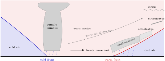
Real fronts have slopes of this order, and the shallow wedge explains their weather. Ahead of a warm front, the warm air glides up a gentle slope for hundreds of kilometres: high clouds, cirrus and cirrostratus, arrive first, then altostratus, and the clouds thicken and lower until rain sets in near the front. A cold front, steeper and faster, up to twice as fast as a warm front, lifts the warm air abruptly: cumulus and cumulonimbus, showers, gusts and a sudden fall of temperature, with pressure that stops falling and starts rising as the front passes. A front where the warm air descends the frontal surface instead of rising up it is called a katafront.

22.2 Extratropical cyclones

Definition 22.4 (Extratropical cyclone; polar-front model; cyclogenesis)

An extratropical cyclone is a cyclone of the middle and high latitudes, often some $2000\,\mathrm{km}$ across, which usually contains fronts, a cold front trailing for hundreds of kilometres towards the equator. The polar-front model describes its life as a wave that grows on the polar front, the long front between polar and tropical air. Cyclogenesis is the formation or the intensification of a cyclone.

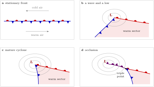
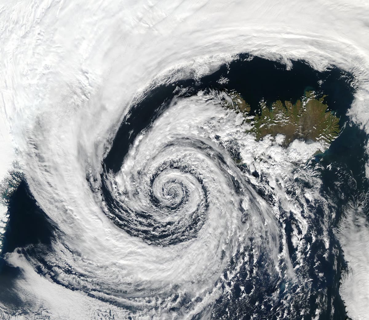
The model follows a cyclone through four stages, as the figure below draws them. A stationary front separates cold air moving west on its polar side from warm air moving east on its equatorial side. A disturbance bends the front into a wave; the pressure falls at its crest, a low forms, and the front east of the low advances poleward as a warm front while the front west of it advances equatorward as a cold front. Between them lies the warm sector. The cold front moves faster than the warm front, the warm sector narrows, and the cold front overtakes the warm front near the low: the occlusion spreads outward from the centre, lifting the warm air off the ground, and the cyclone, cut off from its supply of warm air, fills and dies. The point where the three fronts meet is called the triple point. On satellite images a mature cyclone shows a comma-shaped cloud, and a dry slot of clear air wrapping into its southern and eastern side.

The fronts of the model are only the surface trace of the airflows of the cyclone, which meteorologists describe as three streams: a warm conveyor belt, the moist air that rises from the warm sector ahead of the cold front; a cold conveyor belt on the cold side of the fronts; and a dry intrusion, a stream of air from the upper troposphere, sometimes from the lowest stratosphere, that descends towards the surface behind the cold front and fans out near the ground.

Where does the energy of a cyclone come from? Not from latent heat alone, as in a thunderstorm, but from the contrast of temperature between polar and tropical air. Mid-latitude cyclones strengthen in baroclinic zones, where the temperature changes horizontally on a surface of constant pressure and the wind changes with height. A growing cyclone carries warm air poleward and upward and cold air equatorward and downward: it lowers the centre of mass of the atmosphere and converts potential energy into the kinetic energy of its winds. The Year 3 volume studies that conversion.

22.3 Jet streams and Rossby waves

Cyclones are not scattered at random. The polar jet, the fast core of the westerlies above the polar front, goes with the position and the motion of the highs and lows of the middle latitudes; it is fastest along its jet streaks, the stretches where its wind speed peaks, and it does not circle the pole as a ring: it meanders.

Definition 22.5 (Rossby wave; upper-level trough and ridge)

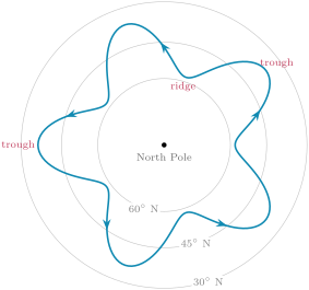
A Rossby wave is a wave of the westerly flow of the upper troposphere, a series of troughs and ridges thousands of kilometres long with a large north–south amplitude. An upper-level trough is an elongated region of relatively low pressure in such a wave, where the flow bends towards the equator; an upper-level ridge is an elongated region of relatively high pressure, where it bends towards the pole.

Rossby waves exist because the Coriolis parameter grows towards the pole. Air pushed poleward finds a larger $f$ and, conserving its absolute vorticity, turns back towards the equator; air pushed equatorward turns back towards the pole. The rate at which $f$ grows northward, $\beta = \mathrm{d}f/\mathrm{d}y = 2\Omega\cos\varphi/a$ with $a$ the radius of the Earth, sets their speed. The Year 3 volume derives, from the conservation of vorticity, the phase speed of a wave of wavelength $\lambda$ in a uniform westerly wind $U$:

Admit it here. Relative to the air, every Rossby wave moves west, and the longer the wave, the faster; the wind carries it east. Short waves are carried east almost at the speed of the wind, long ones drift slowly, stand still, or even move west.

Example 22.6 (Three waves at 45° N)

With $\Omega = 7.292 \times 10^{-5}\,\mathrm{s}^{-1}$ (a sidereal day of $23.9345\,\mathrm{h}$) and $a = 6371\,\mathrm{km}$, $\beta = 1.62 \times 10^{-11}\,\mathrm{m}^{-1}\,\mathrm{s}^{-1}$ at $45{}^{\circ}$ N. In a westerly of $15\,\mathrm{m}/\mathrm{s}$, a wave of $4000\,\mathrm{km}$ has $\beta/k^2 = 6.6\,\mathrm{m}/\mathrm{s}$ and moves east at $8.4\,\mathrm{m}/\mathrm{s}$; one of $6000\,\mathrm{km}$ has $\beta/k^2 = 14.8\,\mathrm{m}/\mathrm{s}$ and barely moves, at $0.2\,\mathrm{m}/\mathrm{s}$; one of $8000\,\mathrm{km}$ moves west at $11.2\,\mathrm{m}/\mathrm{s}$.

The troughs of the long waves move slowly and last long; the short waves that travel through them, shortwave troughs, induce rising air ahead of them, on their eastern side, where the surface pressure falls and lows develop. A trough whose axis tilts from south-east to north-west is often a sign of a developing or intensifying system.

Sometimes the pattern stops moving altogether.

Definition 22.7 (Atmospheric blocking)

Atmospheric blocking is a large, persistent and nearly stationary high-pressure system, sometimes paired with a low, that interrupts the normal eastward flow of the jet stream. Methods of detecting blocks almost all require it to last at least five days.

A block diverts the jet and the cyclones around it and holds the same weather over the same region for days: blocks bring heat waves, droughts, wildfires, cold spells and floods to the middle latitudes. In late June and early July 2021 a strong block led to the heat wave of the Pacific Northwest of North America, which caused more than a thousand deaths. The physical processes behind blocking are still not well understood, and numerical models struggle to reproduce how often blocks occur and how long they last.

22.4 Tropical cyclones

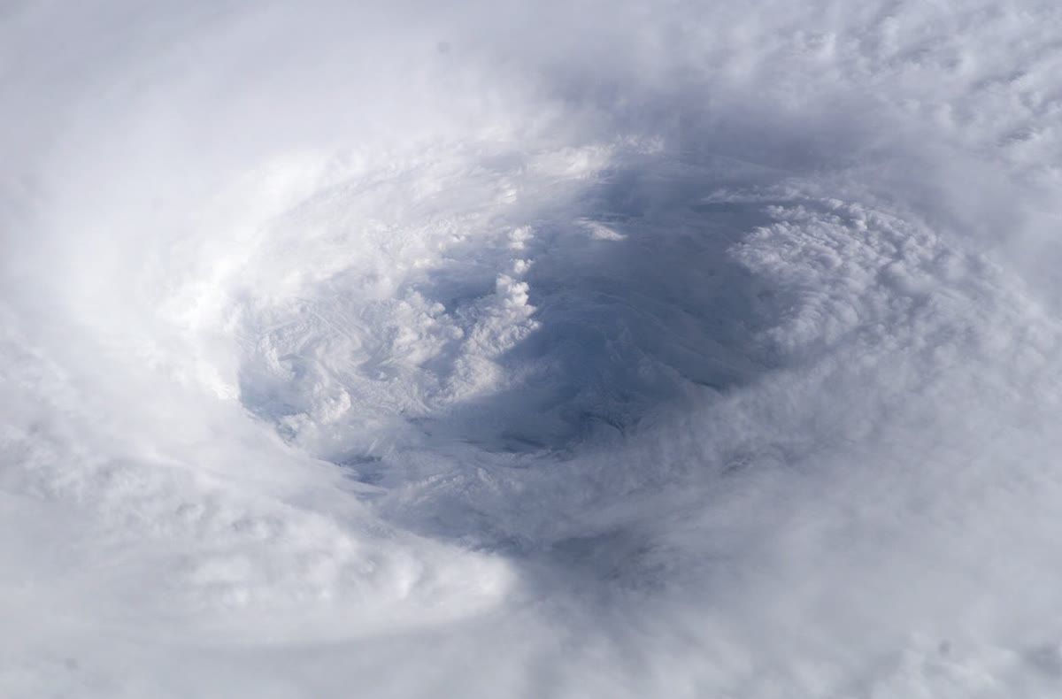
Tropical cyclones have no fronts and no temperature contrast to feed on. They draw their energy from the warm ocean, through the latent heat of the water they evaporate, as Chapter 21 measured it. Six conditions favour their formation: ocean water of at least $26.5\,{}^{\circ}\mathrm{C}$ through a depth of the order of $50\,\mathrm{m}$; an atmosphere that cools fast enough with height to be unstable for moist convection; a moist middle troposphere, around $5\,\mathrm{km}$; a distance of at least about $500\,\mathrm{km}$ from the equator, so that the Coriolis force can hold the low in balance; a pre-existing disturbance near the surface; and weak vertical wind shear, below about $10\,\mathrm{m}/\mathrm{s}$ between the surface and the upper troposphere. They are necessary but not sufficient: many disturbances that meet them never develop.

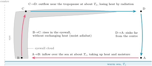
Once formed, a tropical cyclone is a heat engine. Air spirals inward over the sea at almost constant temperature, gaining heat and moisture from the ocean; in the eyewall it rises adiabatically; in the outflow near the tropopause it loses heat by radiation at a low, almost constant temperature; and it sinks again far from the centre, completing a cycle that resembles that of Carnot. The work of the cycle drives the winds against the friction of the sea surface.

Proposition 22.8 (Potential intensity)

The potential intensity of a tropical cyclone, the maximum wind speed near the surface that the ocean and atmosphere around it can sustain, is approximately given by

$$V_{\max}^2 = \frac{C_k}{C_D}\,\frac{T_s - T_o}{T_o}\,\bigl(h_o^* - h^*\bigr),$$

where $T_s$ is the temperature of the sea surface, $T_o$ the temperature of the outflow, $C_k/C_D$ the ratio of the exchange coefficients of enthalpy and momentum between the sea and the air, usually taken as 0.9, and $h_o^* - h^*$ the excess of $c_pT + gz + Lq$ at saturation at the sea surface over its saturation value in the air above the boundary layer (admitted).

The fraction $(T_s - T_o)/T_o$ is not the Carnot efficiency $(T_s - T_o)/T_s$ of the physics books: it is larger by the factor $T_s/T_o$, because the friction that dissipates the work heats the inflowing air near the sea surface, and that heat is used again by the engine. The last factor is the fuel. In a tropical atmosphere whose temperature follows the moist adiabat of its boundary-layer air, $h^*$ is the value of $c_pT + gz + Lq$ in that air, and $h_o^* - h^*$ measures how far the air over the sea is from saturation at the temperature of the sea:

with $T_a$ and $q_a$ the temperature and specific humidity of the air near the surface and $q_s^*$ the saturation specific humidity at the sea-surface temperature.

Example 22.9 (A potential intensity)

Over a sea at $29\,{}^{\circ}\mathrm{C}$ the air at $1015\,\mathrm{hPa}$ is at $28\,{}^{\circ}\mathrm{C}$ with a relative humidity of $80\,\%$, and the outflow is at $200\,\mathrm{K}$, a typical annual mean over the warm tropical oceans. By Propositions 21.5 and 21.2, $e_s(29\,{}^{\circ}\mathrm{C}) = 41.0\,\mathrm{hPa}$, so $q_s^* = 25.5\,\mathrm{g}/\mathrm{kg}$, and the air, with $e = 0.8 \times 38.7\,\mathrm{hPa}$, has $q_a = 19.2\,\mathrm{g}/\mathrm{kg}$. Then $h_o^* - h^* = 1004.5 \times 1 + 2.501 \times 10^6 \times 0.0063 = 16.8\,\mathrm{kJ}/\mathrm{kg}$, the factor $(T_s - T_o)/T_o$ is $(302.15 - 200)/200 = 0.511$, and $V_{\max} = \sqrt{0.9 \times 0.511 \times 16\,800} = 88\,\mathrm{m}/\mathrm{s}$.

The strongest storms come close to such values: the top of the Saffir–Simpson scale, category 5, starts at $70\,\mathrm{m}/\mathrm{s}$, and five recent storms have exceeded $86\,\mathrm{m}/\mathrm{s}$. Most storms rarely reach their potential intensity: real storms are seldom in the steady state the theory assumes, and the theory leaves out vertical wind shear, dry air drawn into the storm and the sinking of the air around it, which weaken a storm.

22.5 Numerical weather prediction

Definition 22.10 (Numerical weather prediction; data assimilation; ensemble forecast; predictability limit)

Numerical weather prediction is forecasting by computer: the equations that govern the motion, the energy and the water of the atmosphere are integrated forward in time from its observed state. Data assimilation combines the latest observations with a short-range forecast from earlier observations to obtain the best estimate of the present state, the analysis, from which the forecast starts. An ensemble forecast is a set of forecasts run from slightly different initial states, and with slightly different versions of the model, to show the range of possible weather and its likelihood. The predictability limit is the time beyond which a forecast of the state of the weather is no better than a guess from climate, because the errors of the initial state have grown as large as the differences between any two states of the atmosphere.

The first numerical forecast was computed in 1950 on ENIAC, one of the first electronic computers. A global model today divides the atmosphere into a grid of cells some kilometres across and starts from an analysis that blends observations from weather stations, aircraft, radiosondes, ships, buoys and, above all, satellites, which bring the largest contribution to the skill of global forecasts. At one large forecast centre the ensemble has 51 members, a control run and 50 perturbed ones, at a resolution of about $9\,\mathrm{km}$, run twice a day to 15 days ahead.

Why perturb a forecast that could start from the best analysis? Because the atmosphere is chaotic, sensitive to its initial state. A system of three variables, published in 1963, shows it at the smallest scale.

Proposition 22.11 (The Lorenz system)

The system

$$\dot x = \sigma(y - x), \qquad \dot y = x(r - z) - y, \qquad \dot z = xy - bz,$$

with $\sigma = 10$, $r = 28$ and $b = 8/3$, has the following properties.

1. Its fixed points are the origin and $C_\pm = \bigl(\pm\sqrt{b(r - 1)}, \pm\sqrt{b(r - 1)}, r - 1\bigr) = (\pm 8.49, \pm 8.49, 27)$.
2. Every volume in its phase space shrinks as $\mathrm{e}^{-(\sigma + 1 + b)t}$: its trajectories end on a set of zero volume, the attractor.
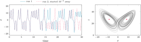
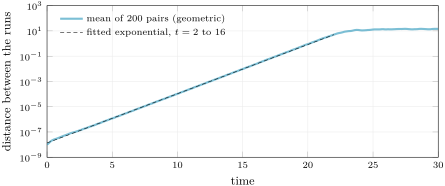
3. On the attractor, two trajectories that start a small distance $\delta_0$ apart separate, on average, as $\delta(t) \approx \delta_0\,\mathrm{e}^{\lambda t}$, with $\lambda = 0.906$, until $\delta$ reaches the size of the attractor (computed, admitted). Small errors double every $\ln 2/\lambda = 0.77$ time units.

The figures show what the proposition means. Two runs that start $10^{-5}$ apart follow each other for some fifteen time units, then part for good: each still looks like a plausible trajectory of the system, but they are no longer the same trajectory. Averaged over 200 pairs of runs started $10^{-8}$ apart, the distance grows exponentially at the rate $\lambda$, a straight line on a logarithmic scale, until it saturates at the size of the attractor. Whatever the initial error, it reaches that size: a smaller initial error only delays the moment, by $\ln 10/\lambda = 2.5$ time units for each tenfold reduction.

The atmosphere behaves in the same way, with many more variables and with errors that grow at different rates on different scales. From the forecasts of the 1980s, small errors were found to double in about 2.4 days, and the reliable forecast of the state of the weather stops short of about ten days. Experiments that shrink today’s uncertainty of the initial state, with a model assumed perfect, find that perfect initial conditions would add only four to five days, and that a 90 per cent reduction already gives nearly all of it: as the errors get smaller, they grow faster, through the release of latent heat in convection, on scales smaller than the forecast can resolve. The predictability limit of the middle latitudes lies around two weeks. Forecasts gain about a day per decade because better observations, assimilation and models move them closer to that limit; they cannot cross it.

The ensemble turns this into a tool. Its members start from analyses that differ by about as much as the analysis itself is uncertain; while they agree, the forecast is sharp; when they spread, the forecast must say so, and it gives probabilities. A forecast is called reliable when the events it announces with a probability of $70\,\%$ happen in $70\,\%$ of the cases.

In the lab — A day at a forecast centre

At a global forecast centre the day turns around two times, 00 and 12 UTC. Observations valid around each time arrive in their millions, from satellites, radiosondes, aircraft, ships and buoys and weather stations; data assimilation blends them with the previous short forecast into the analysis. The models start from it, the ensemble too, and the forecasts reach their users several hours later, after the supercomputers have run the 15 days ahead. Forecasters then compare the runs, check them against the latest observations and the satellite images, follow the cyclones and the fronts, and turn the probabilities of the ensemble into warnings and forecasts.

Exercises

Data for the exercises, unless stated otherwise: $\Omega = 7.292 \times 10^{-5}\,\mathrm{s}^{-1}$, $a = 6371\,\mathrm{km}$, $g = 9.81\,\mathrm{m}\,\mathrm{s}^{-2}$, $c_p = 1004.5\,\mathrm{J}\,\mathrm{kg}^{-1}\,\mathrm{K}^{-1}$, $L = 2.501 \times 10^{6}\,\mathrm{J}/\mathrm{kg}$, and the saturation vapour pressure of the exercises of Chapter 21.

Exercise 22.1 ★

At $50{}^{\circ}$ N a cold front separates air at $275\,\mathrm{K}$ from air at $281\,\mathrm{K}$, and the wind along it changes by $15\,\mathrm{m}/\mathrm{s}$. (a) Compute $f$. (b) Compute the slope of the frontal surface, as 1 in $N$. (c) How far behind the front on the ground does the frontal surface reach $1\,\mathrm{km}$? (d) What happens to the slope if the temperature contrast doubles at the same wind shift?

Solution

Solution of Exercise 22.1.

(a) $f = 2 \times 7.292 \times 10^{-5} \times \sin50{}^{\circ} = 1.117 \times 10^{-4}\,\mathrm{s}^{-1}$. (b) With $\bar T = 278\,\mathrm{K}$, $\tan\alpha = 1.117 \times 10^{-4} \times 278 \times 15/(9.81 \times 6) = 0.00791$, about 1 in 126. (c) $1/0.00791 = 126$: some $126\,\mathrm{km}$ behind the front. (d) The slope is inversely proportional to the temperature contrast: it halves, to 1 in 253.

Exercise 22.2 ★

A warm frontal surface rises at 1 in 150 and moves at $25\,\mathrm{km}/\mathrm{h}$. (a) How far ahead of the front on the ground is the frontal surface $6\,\mathrm{km}$ up? (b) An observer sees high cloud form on it there. How long after does the front reach the observer? (c) Describe the sequence of clouds the observer sees meanwhile.

Solution

Solution of Exercise 22.2.

(a) $6 \times 150 = 900\,\mathrm{km}$ ahead. (b) $900/25 = 36\,\mathrm{h}$, a day and a half. (c) First the high cirrus, then cirrostratus, then altostratus; the cloud thickens and lowers, and rain sets in from the low, thick cloud as the front comes near.

Exercise 22.3 ★

On a Northern Hemisphere map, (a) a line with blue triangles on its south-east side runs south-west from a low; (b) a line with red semicircles on its north side runs east from the same low; (c) a purple line with both symbols runs from another low to a point where two other fronts start; (d) a line alternates blue triangles on its south side and red semicircles on its north side. Name each front, say where the cold air is and which way each moves.

Solution

Solution of Exercise 22.3.

The symbols point the way the front moves, and into the warmer air ahead of a cold front or the colder air ahead of a warm front. (a) A cold front: the cold air lies to its north-west, behind it; it moves south-east. (b) A warm front: the cold air lies to its north, ahead of it; it moves north. (c) An occluded front, joining the low to the triple point where the cold and warm fronts start; cold air lies on both sides of it, the warm air lifted above; it moves the way its symbols point. (d) A stationary front: the triangles point south into the warm air, so the cold air lies to the north; it barely moves.

Exercise 22.4 ★

At $45{}^{\circ}$ N in a westerly of $12\,\mathrm{m}/\mathrm{s}$: (a) compute $\beta$. (b) Compute the phase speed of waves of $4000\,\mathrm{km}$ and $8000\,\mathrm{km}$. (c) Which way does each move, and how far in a day?

Solution

Solution of Exercise 22.4.

(a) $\beta = 2 \times 7.292 \times 10^{-5} \times \cos45{}^{\circ}/(6.371 \times 10^6) = 1.62 \times 10^{-11}\,\mathrm{m}^{-1}\,\mathrm{s}^{-1}$. (b) For $4000\,\mathrm{km}$, $k = 1.571 \times 10^{-6}\,\mathrm{m}^{-1}$, $\beta/k^2 = 6.6\,\mathrm{m}/\mathrm{s}$ and $c = 12 - 6.6 = 5.4\,\mathrm{m}/\mathrm{s}$; for $8000\,\mathrm{km}$, $\beta/k^2 = 26.3\,\mathrm{m}/\mathrm{s}$ and $c = -14.3\,\mathrm{m}/\mathrm{s}$. (c) The short wave moves east, $470\,\mathrm{km}$ a day; the long one moves west, $1240\,\mathrm{km}$ a day, against the wind.

Exercise 22.5 ★★

(a) Show that a Rossby wave stands still in a westerly $U$ when $\lambda = 2\pi\sqrt{U/\beta}$. (b) Compute it at $45{}^{\circ}$ N for $U = 12\,\mathrm{m}/\mathrm{s}$. (c) How many such waves fit round the latitude circle? (d) Why would a stronger westerly favour fewer, longer standing waves?

Solution

Solution of Exercise 22.5.

(a) $c = 0$ when $U = \beta/k^2$, so $k = \sqrt{\beta/U}$ and $\lambda = 2\pi/k = 2\pi\sqrt{U/\beta}$. (b) $2\pi\sqrt{12/(1.62 \times 10^{-11})} = 5410\,\mathrm{km}$. (c) The circle of latitude $45{}^{\circ}$ measures $2\pi \times 6371 \times \cos45{}^{\circ} = 28\,300\,\mathrm{km}$: about 5.2 waves, so five in practice. (d) $\lambda$ grows as $\sqrt U$: a stronger westerly makes the standing waves longer, and fewer of them fit round the hemisphere.

Exercise 22.6 ★★

For the Lorenz system: (a) check that $C_+$ is a fixed point by computing the three derivatives there. (b) By what factor does a small volume of phase space shrink in one time unit? (c) Why does this not prevent two nearby trajectories from separating?

Solution

Solution of Exercise 22.6.

(a) At $C_+ = (\sqrt{72}, \sqrt{72}, 27)$: $\dot x = 10(\sqrt{72} - \sqrt{72}) = 0$, $\dot y = \sqrt{72}(28 - 27) - \sqrt{72} = 0$, $\dot z = 72 - \tfrac83 \times 27 = 72 - 72 = 0$. (b) $\mathrm{e}^{-13.67} = 1.16 \times 10^{-6}$: the volume shrinks almost a millionfold in one time unit. (c) A volume can shrink while it is stretched in one direction and squeezed much more strongly in the others: the distance along the stretched direction grows, and two nearby trajectories separate along it, while the volume between them vanishes.

Exercise 22.7 ★★

Take $\lambda = 0.906$ for the Lorenz system and an attractor of size 10. (a) Compute the doubling time of small errors. (b) How long does an error of $10^{-8}$ take to reach the size of the attractor? (c) By how much does a thousandfold smaller initial error delay that moment? What fraction of the time found in (b) is that?

Solution

Solution of Exercise 22.7.

(a) $\ln 2/0.906 = 0.765$ time units. (b) $\ln(10/10^{-8})/0.906 = \ln(10^9)/0.906 = 22.9$ time units. (c) $\ln 1000/0.906 = 7.6$ time units: a thousandfold improvement of the initial state buys only a third of the time found in (b), since $\ln 10^3/\ln 10^9 = 1/3$.

Exercise 22.8 ★★

A sea at $303\,\mathrm{K}$ has an outflow at $195\,\mathrm{K}$; the disequilibrium is $h_o^* - h^* = 15\,\mathrm{kJ}/\mathrm{kg}$ and $C_k/C_D = 0.9$. (a) Compute the potential intensity. (b) Compare it with the threshold of category 5 and with the fastest recent storms. (c) Why do most storms not reach it?

Solution

Solution of Exercise 22.8.

(a) $(303 - 195)/195 = 0.554$ and $V_{\max} = \sqrt{0.9 \times 0.554 \times 15\,000} = 86.5\,\mathrm{m}/\mathrm{s}$. (b) Well above the $70\,\mathrm{m}/\mathrm{s}$ of category 5, close to the $86\,\mathrm{m}/\mathrm{s}$ that five recent storms have exceeded. (c) Storms rarely stay long in the steady state the theory assumes; vertical wind shear, dry air drawn into the storm and the sinking air around it, which the theory leaves out, weaken them.

Exercise 22.9 ★★

For the storm of Exercise 22.8: (a) compute the Carnot efficiency of an engine working between the sea surface and the outflow. (b) Compute the factor $(T_s - T_o)/T_o$ of Proposition 22.8 and the ratio of the two. (c) Explain the difference.

Solution

Solution of Exercise 22.9.

(a) $(303 - 195)/303 = 0.356$. (b) $(303 - 195)/195 = 0.554$; the ratio is $0.554/0.356 = 303/195 = 1.554$. (c) In a Carnot engine the work leaves the engine. In a tropical cyclone the work is dissipated by friction near the sea surface, and that heat warms the inflowing air at the temperature $T_s$, where the engine takes in its heat: it is used again, and the engine behaves as if it were more efficient by the factor $T_s/T_o$.

Exercise 22.10 ★★★

(a) Rederive Proposition 22.2, keeping the densities exact, and show that the cold air must lie beneath. (b) Across a frontal zone $50\,\mathrm{km}$ wide at $45{}^{\circ}$ N the wind along the front changes by $10\,\mathrm{m}/\mathrm{s}$. Compute the relative vorticity of the zone and compare it with $f$. (c) Is the zone cyclonic or anticyclonic?

Solution

Solution of Exercise 22.10.

(a) The derivation of Proposition 22.2 without approximation gives $\mathrm{d}z/\mathrm{d}x = f(\rho_c v_c - \rho_w v_w)/[g(\rho_c - \rho_w)]$. A denser fluid resting on a lighter one is unstable: the slightest disturbance makes it overturn. In a front at rest the cold, denser air must therefore lie beneath, which is the wedge of the definition; then $\rho_c > \rho_w$, the surface rises towards the cold air, and $\rho_c v_c > \rho_w v_w$. (b) $\zeta = \partial v/\partial x = 10/(50 \times 10^3) = 2 \times 10^{-4}\,\mathrm{s}^{-1}$, about $1.9f$ with $f = 1.03 \times 10^{-4}\,\mathrm{s}^{-1}$. (c) Positive in the Northern Hemisphere: cyclonic, and as large as the Coriolis parameter itself; fronts are bands of strong cyclonic vorticity.

Exercise 22.11 ★★★

Suppose forecast errors double every 2.4 days, start at $0.5\,\mathrm{K}$ and are useless at $6\,\mathrm{K}$. (a) Find the horizon of useful forecasts. (b) By what factor must the initial error shrink each decade to gain a day per decade, if the model were perfect? (c) Experiments find that a tenfold smaller initial error gains only 4 to 5 days. What doubling time does that imply for small errors, and what does it say about how small errors grow?

Solution

Solution of Exercise 22.11.

(a) $\log_2(6/0.5) = \log_2 12 = 3.58$ doublings, $3.58 \times 2.4 = 8.6$ days. (b) One more day of forecast needs one doubling time less of growth before the error is useless: the initial error must shrink by $2^{1/2.4} = 1.33$ each decade. (c) A tenfold reduction is $\log_2 10 = 3.32$ doublings; if it gains only 4 to 5 days, small errors double in $4/3.32 = 1.2$ to $5/3.32 = 1.5$ days: smaller errors grow faster than the larger ones measured in the forecasts of the 1980s, through latent heat released in convection on small scales.

Exercise 22.12 ★★★

Take Example 22.9 and warm both the sea and the air by $1\,\mathrm{K}$, the relative humidity and the outflow temperature unchanged. (a) Recompute $q_s^*$, $q_a$ and the disequilibrium. (b) Recompute the potential intensity. (c) By how many per cent per kelvin does it rise, and which factor contributes most?

Solution

Solution of Exercise 22.12.

(a) At $30\,{}^{\circ}\mathrm{C}$, $e_s = 43.5\,\mathrm{hPa}$ and $q_s^* = 27.1\,\mathrm{g}/\mathrm{kg}$; the air at $29\,{}^{\circ}\mathrm{C}$ has $e = 0.8 \times 41.0 = 32.8\,\mathrm{hPa}$ and $q_a = 20.4\,\mathrm{g}/\mathrm{kg}$; $h_o^* - h^* = 1004.5 \times 1 + 2.501 \times 10^6 \times 0.0067 = 17.8\,\mathrm{kJ}/\mathrm{kg}$, against $16.8\,\mathrm{kJ}/\mathrm{kg}$. (b) $(303.15 - 200)/200 = 0.516$ and $V_{\max} = \sqrt{0.9 \times 0.516 \times 17\,800} = 90.9\,\mathrm{m}/\mathrm{s}$, against $87.9\,\mathrm{m}/\mathrm{s}$. (c) About $3.4\,\%$ per kelvin. The disequilibrium rises by $6\,\%$, which adds $3\,\%$ to the speed; the factor $(T_s - T_o)/T_o$ rises by $1\,\%$, which adds $0.5\,\%$: the fuel, the moisture the warmer sea can give, contributes most, through the exponential rise of $e_s$.

Problem 22.1

Weekend problem — How far ahead?

An invented weather chart at $50{}^{\circ}$ N shows a cold front advancing on a town, with a Rossby wave in the jet stream above. The problem follows the front, then the wave, then asks how far ahead any of it can be forecast. Use the data of the exercises.

Part I — The front. At 06 UTC the cold front is $480\,\mathrm{km}$ west of the town, at 12 UTC $390\,\mathrm{km}$. Behind it the air is at $277\,\mathrm{K}$, in the warm sector at $285\,\mathrm{K}$, and the wind along the front changes by $16\,\mathrm{m}/\mathrm{s}$ across it.

1. Find the speed of the front.
2. At what time does it reach the town?
3. Compute $f$ at $50{}^{\circ}$ N.
4. Compute the slope of the frontal surface.
5. How high is the frontal surface above the town six hours after the front has passed?
6. How long after the passage does the cold air reach $1.5\,\mathrm{km}$ above the town?
7. What weather does the town see as the front passes, and how does the pressure change?

Part II — The wave aloft. In the jet above, the westerly is $20\,\mathrm{m}/\mathrm{s}$ and the wave has a wavelength of $5000\,\mathrm{km}$.

8. Compute $\beta$ at $50{}^{\circ}$ N.
9. Compute $k$ and $\beta/k^2$.
10. Find the phase speed of the wave.
11. How far does a trough move in 24 hours?
12. Find the wavelength that would stand still in this wind, and how many such waves fit round $50{}^{\circ}$ N.
13. Where, relative to the upper trough, should the surface cyclone deepen?

Part III — A toy atmosphere. In the figure of the growth of errors in the Lorenz system, the fitted line passes through about $5 \times 10^{-7}$ at $t = 4$ and $3.9 \times 10^{-3}$ at $t = 14$.

14. From these two readings, compute the growth rate $\lambda$.
15. Compute the doubling time.
16. Compare with the published exponent 0.906.
17. Why does the distance stop growing, at about 15?
18. How much later does an error ten times smaller reach that size?

Part IV — How far ahead? Take the doubling time of 2.4 days found for small errors of the forecasts of the 1980s, an initial error of $0.1\,{}^{\circ}\mathrm{C}$ in the temperature at some level, and a forecast that is useless once the error reaches $3\,{}^{\circ}\mathrm{C}$.

19. How many doublings separate the initial error from the useless one?
20. How many days does that take?
21. How many days would halving the initial error gain?
22. With the earlier estimate of a doubling time of 5 days, what horizon would one find?
23. Modern experiments find that a tenfold smaller initial error, and even a perfect initial state, gains only 4 to 5 days. Why does that suggest that the estimate of question 20 is optimistic?
24. To sum up: how far ahead, in days, could this forecast be useful?

Solution

Solution of Problem 22.1.

1. $(480 - 390)/6 = 15\,\mathrm{km}/\mathrm{h}$. 2. $390/15 = 26\,\mathrm{h}$ after 12 UTC: at 14 UTC the next day. 3. $f = 1.117 \times 10^{-4}\,\mathrm{s}^{-1}$. 4. With $\bar T = 281\,\mathrm{K}$, $\tan\alpha = 1.117 \times 10^{-4} \times 281 \times 16/(9.81 \times 8) = 0.0064$, about 1 in 156. 5. The front is then $6 \times 15 = 90\,\mathrm{km}$ beyond the town; the surface is $90\,000 \times 0.0064 = 576\,\mathrm{m}$ above it. 6. $1500/0.0064 = 234\,\mathrm{km}$ behind the front, reached $234/15 = 15.6\,\mathrm{h}$ after the passage. 7. Cumulus and cumulonimbus, showers, perhaps thunder, gusts and a sudden fall of temperature; the pressure, falling as the front approaches, starts to rise as it passes; then cooler, clearer air. 8. $\beta = 2 \times 7.292 \times 10^{-5} \times \cos50{}^{\circ}/(6.371 \times 10^6) = 1.47 \times 10^{-11}\,\mathrm{m}^{-1}\,\mathrm{s}^{-1}$. 9. $k = 2\pi/(5 \times 10^6) = 1.257 \times 10^{-6}\,\mathrm{m}^{-1}$ and $\beta/k^2 = 9.3\,\mathrm{m}/\mathrm{s}$. 10. $c = 20 - 9.3 = 10.7\,\mathrm{m}/\mathrm{s}$, eastward. 11. $10.7 \times 86\,400 = 924\,\mathrm{km}$ east. 12. $\lambda_s = 2\pi\sqrt{20/(1.47 \times 10^{-11})} = 7330\,\mathrm{km}$; the circle of latitude $50{}^{\circ}$ measures $2\pi \times 6371 \times \cos50{}^{\circ} = 25\,700\,\mathrm{km}$, about 3.5 such waves. 13. Ahead of it, on its eastern side, where the short waves induce rising air and the surface pressure falls. 14. $\lambda = \ln(3.9 \times 10^{-3}/5 \times 10^{-7})/(14 - 4) = \ln 7800/10 = 0.896$. 15. $\ln 2/0.896 = 0.77$ time units. 16. $1\,\%$ below 0.906: the mean of 200 pairs, a finite time and readings from a graph. 17. Once the two runs are far apart, they lie at unrelated points of the attractor, and their distance cannot exceed its size: the growth saturates. 18. $\ln 10/0.896 = 2.6$ time units later. 19. $\log_2(3/0.1) = \log_2 30 = 4.91$ doublings. 20. $4.91 \times 2.4 = 11.8$ days. 21. One doubling time: 2.4 days. 22. $4.91 \times 5 = 24.5$ days: the early estimate was far too optimistic. 23. With a doubling time of 2.4 days, a tenfold smaller error would gain $3.32 \times 2.4 = 8.0$ days, not 4 to 5: small errors grow faster than 2.4 days per doubling, and an estimate built on that doubling time overstates the horizon. 24. This forecast could be useful for at most about 12 days, and in practice for less.