27Anthropogenic Climate Change

Since 1970 the global surface has warmed faster than in any other fifty-year period of at least the last two thousand years (high confidence). The school volumes told what has changed and why. This chapter turns the account into a budget: how many watts per square metre the human drivers add, how many the warmer planet sends back to space, how much warming each tonne of carbon dioxide buys, and how the rising sea is shared between warming water and melting ice. Each number comes with its uncertainty, in the calibrated language of the assessments.

You already know

From the school volumes: radiative forcing, $3.93\,\mathrm{W}\,\mathrm{m}^{-2}$ for a doubling of carbon dioxide, and its logarithmic law; climate feedback; equilibrium climate sensitivity, best estimate $3\,{}^{\circ}\mathrm{C}$, likely 2.5 to $4\,{}^{\circ}\mathrm{C}$; attribution, emission scenario and projection; the calibrated language: likely 66 to $100\,\%$, very likely 90 to $100\,\%$, a range $[x \text{ to } y]$ being a very likely range. Human influence has warmed the climate by $1.07\,{}^{\circ}\mathrm{C}$ between 1850–1900 and 2010–2019. From the physics books: the black body and the Stefan–Boltzmann law; thermal expansion. From the biology books: the carbon cycle, the airborne fraction, carbon sinks and the carbon budget of the biosphere. From Chapter 26: the slow carbon cycle, which takes back an excess of carbon dioxide only over hundreds of thousands of years.

27.1 Forcing quantified

Definition 27.1 (Effective radiative forcing)

The effective radiative forcing (ERF) of a perturbation — a change in a greenhouse gas, in aerosols, in the Sun — is the change it causes in the net downward flux of radiation at the top of the atmosphere, in $\mathrm{W}\,\mathrm{m}^{-2}$, once the atmosphere, the clouds and the land surface have adjusted to it, but before the global surface temperature has responded. The adjustments counted are those caused by the agent itself, independently of the surface temperature.

The definition draws the line between forcing and response by what depends on the surface temperature, not by speed. The instantaneous forcing of carbon dioxide is the change of flux just after the gas is added; the stratosphere, which then cools within months, changes it a first time; the troposphere, its water vapour and its clouds change it again. For a doubling of carbon dioxide the assessment finds $3.75\,\mathrm{W}\,\mathrm{m}^{-2}$ once the stratosphere has adjusted, and adjustments in the troposphere that partly cancel: $-0.60\,\mathrm{W}\,\mathrm{m}^{-2}$ from its warming, +0.22 from water vapour, +0.45 from clouds and +0.11 from the land surface, $+0.18\,\mathrm{W}\,\mathrm{m}^{-2}$ in all. The ERF is $3.75 + 0.18 = 3.93\,\mathrm{W}\,\mathrm{m}^{-2}$, $6\,\%$ more than the $3.71\,\mathrm{W}\,\mathrm{m}^{-2}$ of the previous assessment (Exercise 27.1).

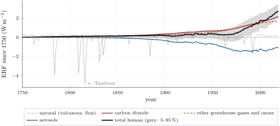
The forcing of every agent since 1750 has been reconstructed year by year. The figure below shows it: carbon dioxide at $2.16\,\mathrm{W}\,\mathrm{m}^{-2}$ in 2019, the other greenhouse gases — methane, nitrous oxide, the halogenated gases and ozone — at $1.69\,\mathrm{W}\,\mathrm{m}^{-2}$ together, and the aerosols at $-1.06\,\mathrm{W}\,\mathrm{m}^{-2}$. The total human forcing is $2.72\,\mathrm{W}\,\mathrm{m}^{-2}$, and its very likely range, 1.96 to $3.48\,\mathrm{W}\,\mathrm{m}^{-2}$, is wide mainly because of the aerosols. Their ERF over 1750–2014 is assessed at $-1.3$ [$-2.0$ to $-0.6$] $\mathrm{W}\,\mathrm{m}^{-2}$ (medium confidence), most of it through their effect on clouds, which brighten when aerosols supply more droplets. Volcanic eruptions add short negative spikes (Chapter 6): the deepest in the record, $-4.8\,\mathrm{W}\,\mathrm{m}^{-2}$ in 1816, follows the eruption of Tambora in 1815.

27.2 The energy budget

A positive forcing makes the planet gain energy. As it warms it radiates more to space, and the gain shrinks; the climate settles only when the two balance.

Definition 27.2 (Earth’s energy imbalance; climate feedback parameter)

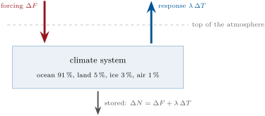
Earth’s energy imbalance $N$ is the net flux of energy into the climate system at the top of the atmosphere, averaged over the globe and over a year or more, in $\mathrm{W}\,\mathrm{m}^{-2}$: absorbed sunlight minus outgoing infrared. It is the rate at which the ocean, the land, the ice and the air gain heat, per square metre of the Earth’s surface.

Definition 27.3 (Climate feedback parameter)

The climate feedback parameter $\lambda$ is the change in the net downward flux at the top of the atmosphere per degree of global surface warming, in $\mathrm{W}\,\mathrm{m}^{-2}\,{}^{\circ}\mathrm{C}^{-1}$, caused by the response of the climate system to that warming. A stable climate has $\lambda < 0$: warming increases the loss of energy to space.

The school volume wrote the balance with the size of $\lambda$, a positive number; from here on the sign is kept, as in the assessments, which write the parameter $\alpha$.

Proposition 27.4 (Global energy balance)

Let $\Delta F$ be the effective radiative forcing and $\Delta T$ the global surface warming relative to an equilibrium state. If the response of the outgoing flux is linear in $\Delta T$,

$$\Delta N = \Delta F + \lambda\,\Delta T .$$

At a new equilibrium $\Delta N = 0$, so $\Delta T_{\text{eq}} = -\Delta F/\lambda$.

Measuring $N$ means measuring the heat the system gains, and the ocean holds nearly all of it. From 1971 to 2018 the climate system gained $435\,\mathrm{ZJ}$ (zettajoules, $10^{21}\,\mathrm{J}$): the ocean $91\,\%$, $242\,\mathrm{ZJ}$ in its top $700\,\mathrm{m}$ and $154\,\mathrm{ZJ}$ below; the land $5\,\%$, the melting ice $3\,\%$, the atmosphere $1\,\%$. The mean imbalance was $0.57\,\mathrm{W}\,\mathrm{m}^{-2}$ over 1971–2018, and it has grown: $0.79\,\mathrm{W}\,\mathrm{m}^{-2}$ [0.52 to 1.06] over 2006–2018 (Exercise 27.2).

Method 27.5 (A climate sensitivity from the historical energy budget)

1. Choose two periods, a reference close to equilibrium and a recent one; take the change in forcing $\Delta F$, in imbalance $\Delta N$ and in global temperature $\Delta T$.
2. Solve the balance for the feedback parameter: $\lambda = (\Delta N - \Delta F)/\Delta T$.
3. The sensitivity to a doubling is then $-F_{2\times}/\lambda$; the warming at the time of the forcing, scaled to $F_{2\times}$, is $F_{2\times}\Delta T/\Delta F$.

From 1850–1900 to 2006–2019 the assessment takes $\Delta N = 0.59\,\mathrm{W}\,\mathrm{m}^{-2}$, $\Delta T = 1.03\,{}^{\circ}\mathrm{C}$ and $\Delta F = 2.20\,\mathrm{W}\,\mathrm{m}^{-2}$. Then $\lambda = (0.59 - 2.20)/1.03 = -1.56\,\mathrm{W}\,\mathrm{m}^{-2}\,{}^{\circ}\mathrm{C}^{-1}$, and the sensitivity is $3.93/1.56 = 2.5\,{}^{\circ}\mathrm{C}$, the value the assessment finds, with a very likely range of 1.6 to $4.8\,{}^{\circ}\mathrm{C}$. But this is an effective sensitivity, for the feedbacks of the warming so far. The warming has been strongest where feedbacks are most negative, in the western tropical Pacific, and weaker over the eastern Pacific and the Southern Ocean; as that pattern evolves the feedback parameter is expected to become less negative (high confidence), so the long-term sensitivity is higher than the historical estimate (Exercise 27.7).

27.3 Feedbacks and sensitivity

Definition 27.6 (Planck response; water-vapour, lapse-rate and cloud feedbacks)

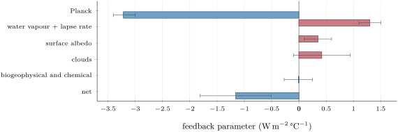
The feedback parameter is split into the contributions of the quantities that change with the surface temperature. The Planck response is the extra infrared emitted to space when the surface and the whole troposphere warm by the same amount. The water-vapour feedback is the change in flux due to the increase of atmospheric water vapour with temperature. The lapse-rate feedback is the change in flux due to a warming that is not uniform with height. The cloud feedback is the change in flux due to the change in the amount, height and brightness of clouds.

Proposition 27.7 (The Planck response)

If the Earth emits to space a fixed fraction $1 - g$ of the infrared $\sigma T^4$ of its surface at temperature $T$, its Planck response is

$$\lambda_{\text P} = -(1 - g)\,4\sigma T^3 .$$

With $g = 0.4$ and $T = 288\,\mathrm{K}$, $\lambda_{\text P} = -3.25\,\mathrm{W}\,\mathrm{m}^{-2}\,\mathrm{K}^{-1}$.

The fraction $g$ is the normalised greenhouse effect: the atmosphere keeps $159\,\mathrm{W}\,\mathrm{m}^{-2}$ of the $398\,\mathrm{W}\,\mathrm{m}^{-2}$ that the surface emits, $g \approx 0.4$. The assessment, with detailed radiation codes, finds $-3.22$ [$-3.4$ to $-3.0$] (high confidence). Water vapour follows the Clausius–Clapeyron law at the global scale, and more vapour absorbs more infrared: the water-vapour feedback is strongly positive, $1.85\,\mathrm{W}\,\mathrm{m}^{-2}\,{}^{\circ}\mathrm{C}^{-1}$ from satellites. In the tropics the upper troposphere warms more than the surface, which then radiates more: the lapse-rate feedback is negative there, positive near the poles, and about $-0.50$ globally. The two are assessed together, $1.30$ [1.1 to 1.5], because what one model puts in one it tends to take from the other. Melting snow and ice darken the surface, +0.35; clouds add $0.42$ [$-0.10$ to $0.94$], the largest uncertainty. A net negative cloud feedback is very unlikely.

Definition 27.8 (Equilibrium climate sensitivity)

The equilibrium climate sensitivity (ECS) is the global surface warming, at the new equilibrium, caused by a doubling of the carbon dioxide of the air from its pre-industrial level, the ice sheets being held fixed.

Proposition 27.9 (Sensitivity and feedback)

If the feedback parameter is constant, $\text{ECS} = -F_{2\times}/\lambda$. With $F_{2\times} = 3.93\,\mathrm{W}\,\mathrm{m}^{-2}$ and the net $\lambda = -1.16\,\mathrm{W}\,\mathrm{m}^{-2}\,{}^{\circ}\mathrm{C}^{-1}$ of the feedbacks above, $\text{ECS} = 3.4\,{}^{\circ}\mathrm{C}$; the Planck response alone would give $3.93/3.22 = 1.2\,{}^{\circ}\mathrm{C}$.

The feedbacks are one line of evidence; the warming since 1850, the energy budget and the climates of the past are others. Combined, they give the assessed ECS of $3\,{}^{\circ}\mathrm{C}$, likely 2.5 to $4\,{}^{\circ}\mathrm{C}$ (high confidence), very likely 2 to $5\,{}^{\circ}\mathrm{C}$. Because the ECS varies as $1/\lambda$, an uncertainty on $\lambda$ that is symmetric gives a range of ECS stretched towards high values (Exercise 27.12).

Definition 27.10 (Transient climate response)

The transient climate response (TCR) is the global surface warming at the moment the carbon dioxide of the air has doubled, when it rises by $1\,\%$ a year from its pre-industrial level, about seventy years after the start.

The TCR is smaller than the ECS because the ocean is still taking up heat when the doubling is reached. Its best estimate is $1.8\,{}^{\circ}\mathrm{C}$, likely 1.4 to $2.2\,{}^{\circ}\mathrm{C}$ (high confidence); the historical energy budget alone gives $3.93 \times 1.03/2.20 = 1.8\,{}^{\circ}\mathrm{C}$ as well.

27.4 Detection and attribution

Definition 27.11 (Detection; attribution; climate fingerprint)

Detection of a climate change is showing that the climate has changed in a defined statistical sense, beyond what its internal variability could produce, without giving the cause. Attribution is evaluating the contributions of several causes to a detected change, with an assigned likelihood. A climate fingerprint is the pattern in space and time of the response to one driver, as simulated by climate models, by which that driver is recognised in the observations.

Different drivers leave different fingerprints. More greenhouse gas warms the troposphere and cools the stratosphere, because a thicker infrared blanket makes the upper layers radiate more to space; a brighter Sun would warm both. The observations show the first pattern: the troposphere has warmed since at least the 1950s, and it is virtually certain that the stratosphere has cooled. It is very likely that the human greenhouse gases were the main driver of the tropospheric warming since 1979, and extremely likely that the depletion of the ozone layer was the main driver of the cooling of the lower stratosphere from 1979 to the mid-1990s.

Method 27.12 (Optimal fingerprinting)

1. Simulate the response to each driver separately: the fingerprints $x_1, \dots, x_k$, as vectors of values in space and time.
2. Write the observations as $y = \sum_i \beta_i x_i + \varepsilon$, with $\varepsilon$ the internal variability, whose statistics are taken from long unforced simulations.
3. Estimate the scaling factors $\beta_i$ by least squares, weighted by the inverse of the variability so that the noisiest components count least, with their confidence intervals.
4. A $\beta_i$ significantly greater than zero means that the response to driver $i$ is detected; an interval that contains 1 and excludes 0 means that the simulated response is consistent with the observations, and the change can be attributed in part to that driver.

Applied to the surface temperature, the method gives the attribution recalled at the start: of the $1.06\,{}^{\circ}\mathrm{C}$ observed between 1850–1900 and 2010–2019, the human influence likely caused 0.8 to $1.3\,{}^{\circ}\mathrm{C}$, best estimate $1.07\,{}^{\circ}\mathrm{C}$; the natural drivers and the internal variability contribute no more than a few tenths of a degree either way (Exercises 27.9 and 27.10).

27.5 Scenarios and cumulative emissions

Definition 27.13 (Shared Socioeconomic Pathway)

A Shared Socioeconomic Pathway (SSP) is one of five narratives of how population, economies and technology might develop over the century. The emission scenarios of the assessment are labelled SSP$x$-$y$: $x$ names the pathway, and $y$ the approximate radiative forcing, in $\mathrm{W}\,\mathrm{m}^{-2}$, that the scenario reaches in 2100.

The five main scenarios run from SSP1-1.9 to SSP5-8.5. The physical science assessment takes them as given: it neither weighs their likelihood nor assesses the narratives. For each, the climate models give a projected warming for 2081–2100 above 1850–1900, from $1.4\,{}^{\circ}\mathrm{C}$ (very likely 1.0 to 1.8) under SSP1-1.9 to $4.4\,{}^{\circ}\mathrm{C}$ (3.3 to 5.7) under SSP5-8.5. The projections share a simple law.

Definition 27.14 (Transient climate response to cumulative CO$_2$ emissions)

The transient climate response to cumulative $\ce{CO2}$ emissions (TCRE) is the global surface warming per unit of carbon dioxide emitted in total since the pre-industrial period, in ${}^{\circ}\mathrm{C}$ per $1000\,\mathrm{Gt}$ of $\ce{CO2}$.

Proposition 27.15 (Warming follows cumulative emissions)

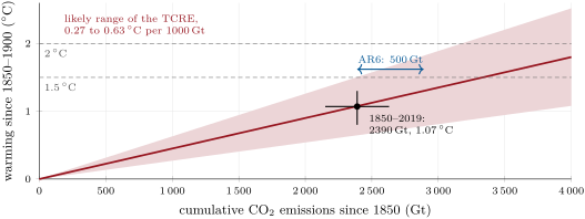
To a good approximation the warming caused by carbon dioxide is proportional to the total emitted, whatever the path of the emissions: $\Delta T \approx \text{TCRE} \times E$, with $E$ the cumulative emissions.

The law is not obvious. The forcing grows only as the logarithm of the concentration, so each added tonne warms less; but the ocean takes up heat and carbon less and less efficiently as emissions accumulate, so more of each tonne stays in the air and its warming is less delayed. The two effects nearly cancel, which all the studies agree is the origin of the law. The relationship is near-linear (high confidence), and each $1000\,\mathrm{Gt}$ of carbon dioxide likely causes 0.27 to $0.63\,{}^{\circ}\mathrm{C}$ of warming, best estimate $0.45\,{}^{\circ}\mathrm{C}$, or $1.65\,{}^{\circ}\mathrm{C}$ per $1000\,\mathrm{PgC}$ of carbon (Exercise 27.4). From 1850 to 2019, $2390 \pm 240\,\mathrm{Gt}$ of carbon dioxide were emitted.

Definition 27.16 (Remaining carbon budget)

The remaining carbon budget for a temperature limit is the cumulative carbon dioxide that can still be emitted, from a stated date, with global warming staying below that limit at a stated probability, the warming caused by the other human drivers being taken into account.

Method 27.17 (The remaining carbon budget from the TCRE)

1. Subtract the human warming already reached, $1.07\,{}^{\circ}\mathrm{C}$ for 2010–2019, from the limit.
2. Subtract the warming the other drivers will add by the time carbon dioxide emissions reach net zero.
3. Divide by the TCRE: this is the budget from the middle of 2010–2019.
4. Subtract the emissions since then, and a margin for the slow Earth-system feedbacks the models leave out (permafrost thaw is the largest).

The assessment combines five components in this way: the TCRE; the historical warming; an additional warming by the other drivers of about 0.1 to $0.2\,{}^{\circ}\mathrm{C}$; the warming that may continue after emissions stop, assessed at zero on average (likely within $\pm 0.19\,{}^{\circ}\mathrm{C}$); and the Earth-system feedbacks, about $26\,\mathrm{Gt}$ of carbon dioxide per degree. For $1.5\,{}^{\circ}\mathrm{C}$, $0.43\,{}^{\circ}\mathrm{C}$ above 2010–2019, the remaining budget from the start of 2020 is $500\,\mathrm{Gt}$ of carbon dioxide at a $50\,\%$ probability, and $1350\,\mathrm{Gt}$ for $2\,{}^{\circ}\mathrm{C}$. The choices made about the other drivers move these values by $220\,\mathrm{Gt}$ or more; the weekend problem rebuilds the first one.

Figures as of 2025

The annual mean carbon dioxide at Mauna Loa reached $427.35\,\mathrm{ppm}$ in 2025, a forcing of $3.93\log_2(427.35/278) = 2.44\,\mathrm{W}\,\mathrm{m}^{-2}$ by the logarithmic law. In the NASA temperature record 2024 is the warmest year, $1.50\,{}^{\circ}\mathrm{C}$ above the mean of 1880–1900, the earliest years of that record; 2025 stood at $1.40\,{}^{\circ}\mathrm{C}$.

27.6 Sea level

Definition 27.18 (Sea-level budget; thermosteric sea-level rise)

The sea-level budget is the comparison of the observed change of global mean sea level with the sum of its estimated contributions: the expansion of the warming ocean, the melting of glaciers and of the Greenland and Antarctic ice sheets, and the change of the water stored on land. Thermosteric sea-level rise is the part due to the thermal expansion of sea water, at constant mass.

Proposition 27.19 (Thermal expansion of a layer)

A layer of ocean of thickness $H$, with thermal expansion coefficient $\alpha$, that warms uniformly by $\Delta T$ at constant mass and area rises by $\Delta h = \alpha\,\Delta T\,H$.

In the real ocean $\alpha$ grows with temperature and pressure, and the warming is concentrated near the surface. The assessment summarises the result as an expansion efficiency of $0.113\,\mathrm{m}$ per $10^{24}\,\mathrm{J}$ of heat added to the ocean, or $0.617\,\mathrm{m}$ per degree of warming of the whole ocean (medium confidence). Over its mean depth of $3682\,\mathrm{m}$, that is an effective $\alpha$ of $0.617/3682 = 1.68 \times 10^{-4}\,{}^{\circ}\mathrm{C}^{-1}$ (Exercise 27.8).

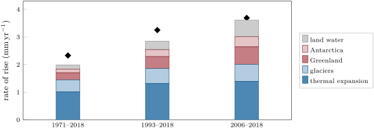
The budget, drawn in the figure below, closes within its uncertainties. Over 1971–2018 the contributions add up to $2.00\,\mathrm{mm}\,\mathrm{yr}^{-1}$, against an observed rise of $2.33\,\mathrm{mm}\,\mathrm{yr}^{-1}$; over 2006–2018 they add up to 3.61 against 3.69. Thermal expansion was the largest single term, half of the sum over 1971–2018, but the ice is catching up: over 2006–2018 glaciers and ice sheets together gave $1.62\,\mathrm{mm}\,\mathrm{yr}^{-1}$, more than the expansion. The ocean also keeps warming at depth long after the surface settles, and the ice sheets respond over centuries; sea level is committed to rise for centuries to millennia and will remain high for thousands of years (high confidence). Over the next two thousand years it is projected to rise by about 2 to $3\,\mathrm{m}$ if the warming stays at $1.5\,{}^{\circ}\mathrm{C}$, 2 to $6\,\mathrm{m}$ at $2\,{}^{\circ}\mathrm{C}$ and 19 to $22\,\mathrm{m}$ at $5\,{}^{\circ}\mathrm{C}$ (low confidence).

Exercises

Data for the exercises, unless stated otherwise: forcing of doubled carbon dioxide $F_{2\times} = 3.93\,\mathrm{W}\,\mathrm{m}^{-2}$ from $C_0 = 278\,\mathrm{ppm}$; Stefan–Boltzmann constant $\sigma = 5.670 \times 10^{-8}\,\mathrm{W}\,\mathrm{m}^{-2}\,\mathrm{K}^{-4}$; radius of the Earth $6371\,\mathrm{km}$; one year $3.156 \times 10^{7}\,\mathrm{s}$; molar masses of carbon and carbon dioxide 12.011 and $44.009\,\mathrm{g}\,\mathrm{mol}^{-1}$; the feedbacks and the sea-level budget of the chapter.

Exercise 27.1 ★

The forcing of doubled carbon dioxide is $3.75\,\mathrm{W}\,\mathrm{m}^{-2}$ once the stratosphere has adjusted; the troposphere then adjusts by $-0.60$ (temperature), +0.22 (water vapour), +0.45 (clouds) and +0.11 (land surface) $\mathrm{W}\,\mathrm{m}^{-2}$. (a) Find the ERF. (b) By what percentage does it exceed the previous assessment’s $3.71\,\mathrm{W}\,\mathrm{m}^{-2}$? (c) Which adjustment is negative, and why does a warmer troposphere reduce the forcing?

Solution

Solution of Exercise 27.1.

(a) $3.75 - 0.60 + 0.22 + 0.45 + 0.11 = 3.93\,\mathrm{W}\,\mathrm{m}^{-2}$, the adjustments adding $0.18\,\mathrm{W}\,\mathrm{m}^{-2}$. (b) $3.93/3.71 = 1.059$: $5.9\,\%$ more. (c) The tropospheric temperature adjustment, $-0.60$: a warmer troposphere emits more infrared to space, which removes part of the extra energy before the surface has responded.

Exercise 27.2 ★

The climate system gained $434.9\,\mathrm{ZJ}$ from 1971 to 2018 and $152.4\,\mathrm{ZJ}$ from 2006 to 2018, counted between the middles of the first and last years. (a) Find the Earth’s surface area. (b) Convert each gain into a mean imbalance in $\mathrm{W}\,\mathrm{m}^{-2}$. (c) The ocean took $91\,\%$: how many zettajoules over 1971–2018?

Solution

Solution of Exercise 27.2.

(a) $4\pi(6.371 \times 10^{6})^2 = 5.10 \times 10^{14}\,\mathrm{m}^{2}$. (b) Over 47 years, $434.9 \times 10^{21}/(47 \times 3.156 \times 10^{7} \times 5.10 \times 10^{14}) = 0.575\,\mathrm{W}\,\mathrm{m}^{-2}$; over 12 years, $152.4 \times 10^{21}/(12 \times 3.156 \times 10^{7} \times 5.10 \times 10^{14}) = 0.789\,\mathrm{W}\,\mathrm{m}^{-2}$, the 0.57 and 0.79 of the assessment. (c) $0.91 \times 434.9 = 396\,\mathrm{ZJ}$.

Exercise 27.3 ★

(a) Add up the central values of the feedbacks in the figure, and compare with the net. (b) Find the ECS with the net value, and the warming with the Planck response alone. (c) By what factor do the other feedbacks amplify the Planck warming?

Solution

Solution of Exercise 27.3.

(a) $-3.22 + 1.30 + 0.35 + 0.42 - 0.01 = -1.16$, the net. (b) $3.93/1.16 = 3.39\,{}^{\circ}\mathrm{C}$; $3.93/3.22 = 1.22\,{}^{\circ}\mathrm{C}$. (c) $3.39/1.22 = 2.78$: the feedbacks almost triple the Planck warming.

Exercise 27.4 ★

(a) Convert a TCRE of $0.45\,{}^{\circ}\mathrm{C}$ per $1000\,\mathrm{Gt}$ of carbon dioxide into degrees per $1000\,\mathrm{PgC}$ of carbon, and do the same for its likely range, 0.27 to 0.63. (b) Convert the $2390\,\mathrm{Gt}$ of carbon dioxide emitted from 1850 to 2019 into petagrams of carbon. (c) What warming does the TCRE give for these emissions?

Solution

Solution of Exercise 27.4.

(a) One petagram of carbon is $44.009/12.011 = 3.664$ Gt of carbon dioxide: $0.45 \times 3.664 = 1.65\,{}^{\circ}\mathrm{C}$ per $1000\,\mathrm{PgC}$, and the range becomes 0.989 to 2.31. (b) $2390 \times 12.011/44.009 = 652\,\mathrm{PgC}$. (c) $0.45 \times 2.39 = 1.08\,{}^{\circ}\mathrm{C}$.

Exercise 27.5 ★★

(a) The surface emits $398\,\mathrm{W}\,\mathrm{m}^{-2}$ and the greenhouse effect keeps $159\,\mathrm{W}\,\mathrm{m}^{-2}$ of it. Find $g$ and the surface temperature of a black body emitting $398\,\mathrm{W}\,\mathrm{m}^{-2}$. (b) Find the Planck response at $288\,\mathrm{K}$, and at $298\,\mathrm{K}$ with the same $g$. (c) Would the Planck response alone make a warmer Earth more or less sensitive?

Solution

Solution of Exercise 27.5.

(a) $g = 159/398 = 0.400$; $T = (398/5.670 \times 10^{-8})^{1/4} = 289\,\mathrm{K}$. (b) $-0.6 \times 4 \times 5.670 \times 10^{-8} \times 288^3 = -3.25\,\mathrm{W}\,\mathrm{m}^{-2}\,\mathrm{K}^{-1}$; at $298\,\mathrm{K}$, $-3.60$. (c) Less sensitive: the response grows as $T^3$, so a warmer planet sheds each extra degree more easily, other feedbacks being equal.

Exercise 27.6 ★★

Satellites give a water-vapour feedback of $1.85 \pm 0.32$ and the studies a lapse-rate feedback of $-0.50 \pm 0.20$ $\mathrm{W}\,\mathrm{m}^{-2}\,{}^{\circ}\mathrm{C}^{-1}$ (one standard deviation). (a) Find their sum. (b) If the two were independent, what would be the standard deviation of the sum? (c) The models give the sum a standard deviation of only $0.10$. What does that say about the two errors?

Solution

Solution of Exercise 27.6.

(a) $1.85 - 0.50 = 1.35\,\mathrm{W}\,\mathrm{m}^{-2}\,{}^{\circ}\mathrm{C}^{-1}$. (b) $\sqrt{0.32^2 + 0.20^2} = 0.38$. (c) The sum is far better known than either term: their errors are strongly anticorrelated. Where the upper troposphere warms more, it also holds more vapour, so a stronger negative lapse-rate feedback comes with a stronger positive water-vapour feedback.

Exercise 27.7 ★★

From 1850–1900 to 2006–2019, $\Delta N = 0.59\,\mathrm{W}\,\mathrm{m}^{-2}$, $\Delta T = 1.03\,{}^{\circ}\mathrm{C}$ and $\Delta F = 2.20\,\mathrm{W}\,\mathrm{m}^{-2}$. (a) Find $\lambda$ and the effective sensitivity. (b) The feedback parameter is expected to become less negative by $\lambda' = 0.5\,\mathrm{W}\,\mathrm{m}^{-2}\,{}^{\circ}\mathrm{C}^{-1}$ as the pattern of warming evolves. Find the sensitivity $-F_{2\times}/(\lambda + \lambda')$. (c) Redo (b) with $\lambda' = 0.1$.

Solution

Solution of Exercise 27.7.

(a) $\lambda = (0.59 - 2.20)/1.03 = -1.56\,\mathrm{W}\,\mathrm{m}^{-2}\,{}^{\circ}\mathrm{C}^{-1}$; $3.93/1.56 = 2.52\,{}^{\circ}\mathrm{C}$. (b) $3.93/(1.56 - 0.5) = 3.93/1.06 = 3.71\,{}^{\circ}\mathrm{C}$. (c) $3.93/1.46 = 2.69\,{}^{\circ}\mathrm{C}$. The assessment, with full distributions, finds 3.5 and $2.7\,{}^{\circ}\mathrm{C}$.

Exercise 27.8 ★★

(a) From the $0.617\,\mathrm{m}$ of rise per degree of warming of the whole ocean, mean depth $3682\,\mathrm{m}$, find the effective expansion coefficient. (b) The ocean gained $396\,\mathrm{ZJ}$ over 1971–2018. With an expansion efficiency of $0.113\,\mathrm{m}$ per $10^{24}\,\mathrm{J}$, find the thermosteric rise, and compare with the $47.5\,\mathrm{mm}$ of the budget. (c) A layer of $700\,\mathrm{m}$ warms by $0.2\,{}^{\circ}\mathrm{C}$ with $\alpha = 2 \times 10^{-4}\,{}^{\circ}\mathrm{C}^{-1}$: how much does it raise sea level?

Solution

Solution of Exercise 27.8.

(a) $0.617/3682 = 1.68 \times 10^{-4}\,{}^{\circ}\mathrm{C}^{-1}$. (b) $0.113 \times 0.396 = 0.0447\,\mathrm{m}$, or $44.7\,\mathrm{mm}$, close to the $47.5\,\mathrm{mm}$ of the budget. (c) $2 \times 10^{-4} \times 0.2 \times 700 = 0.028\,\mathrm{m}$, $28\,\mathrm{mm}$.

Exercise 27.9 ★★

A model fingerprint, in four decades, is $x = (0.10, 0.20, 0.30, 0.40)$ ${}^{\circ}\mathrm{C}$; the observations are $y = (0.12, 0.18, 0.33, 0.41)$ ${}^{\circ}\mathrm{C}$. (a) Find the least-squares scaling factor $\beta$ of $y = \beta x + \varepsilon$. (b) Its standard error, estimated from unforced simulations, is $0.08$. Is the response detected? Is it consistent with the model? (c) What would a $\beta$ of 0.5 with the same error mean?

Solution

Solution of Exercise 27.9.

(a) $\sum xy = 0.311$, $\sum x^2 = 0.300$: $\beta = 1.04$. (b) The $95\,\%$ interval is $1.04 \pm 1.96 \times 0.08$, 0.88 to 1.20: it excludes 0, so the response is detected, and contains 1, so the observed change is consistent with the simulated one. (c) The interval 0.34 to 0.66 still excludes 0 (detected), but excludes 1: the model would overestimate the response by about a factor of two.

Exercise 27.10 ★★★

Two fingerprints, greenhouse gases $g = (0.2, 0.4, 0.6, 0.8)$ and aerosols $a = (-0.1, -0.2, -0.2, -0.3)$, both in ${}^{\circ}\mathrm{C}$ over four decades, are fitted to the observations $y = (0.1, 0.2, 0.4, 0.5)$. (a) Write the normal equations of the least-squares fit $y = \beta_g g + \beta_a a + \varepsilon$ and solve them. (b) Find the warming attributed to each driver in the last decade. (c) Why do the uncertainties on $\beta_g$ and $\beta_a$ grow when the two fingerprints look alike?

Solution

Solution of Exercise 27.10.

(a) $\sum g^2 = 1.20$, $\sum a^2 = 0.18$, $\sum ga = -0.46$, $\sum gy = 0.74$, $\sum ay = -0.28$. The normal equations are $1.20\,\beta_g - 0.46\,\beta_a = 0.74$ and $-0.46\,\beta_g + 0.18\,\beta_a = -0.28$; their determinant is $1.20 \times 0.18 - 0.46^2 = 0.0044$, and $\beta_g = (0.74 \times 0.18 - 0.46 \times 0.28)/0.0044 = 1.00$, $\beta_a = (-1.20 \times 0.28 + 0.46 \times 0.74)/0.0044 = 1.00$. (b) Greenhouse gases $+0.80\,{}^{\circ}\mathrm{C}$, aerosols $-0.30\,{}^{\circ}\mathrm{C}$. (c) The determinant is small because $g$ and $a$ are nearly proportional (their correlation is $-0.99$): a little noise in $y$ can be absorbed by raising both scaling factors together, so each is poorly constrained though their combined effect is well known.

Exercise 27.11 ★★★

Use the method of the remaining carbon budget with the TCRE of $0.45\,{}^{\circ}\mathrm{C}$ per $1000\,\mathrm{Gt}$, the $210\,\mathrm{Gt}$ emitted from 2015 to 2019 and $26\,\mathrm{Gt}$ per degree for the Earth-system feedbacks. (a) Find the budget for $2\,{}^{\circ}\mathrm{C}$, $0.93\,{}^{\circ}\mathrm{C}$ above 2010–2019, if the other drivers add $0.1\,{}^{\circ}\mathrm{C}$. (b) What additional warming by the other drivers makes it equal to the assessed $1350\,\mathrm{Gt}$? Is that within the assessed range? (c) Show that each $0.1\,{}^{\circ}\mathrm{C}$ of non-CO$_2$ warming changes any budget by the same amount.

Solution

Solution of Exercise 27.11.

(a) $(0.93 - 0.1)/0.45 \times 1000 = 1844\,\mathrm{Gt}$; minus 210 and $26 \times 0.93 = 24$: $1610\,\mathrm{Gt}$. (b) $0.93 - x = 0.45 \times (1350 + 210 + 24)/1000 = 0.713$, so $x = 0.22\,{}^{\circ}\mathrm{C}$: about the upper end of the assessed 0.1 to $0.2\,{}^{\circ}\mathrm{C}$. (c) The budget depends on the non-CO$_2$ warming $x$ only through $-x/\text{TCRE}$: each $0.1\,{}^{\circ}\mathrm{C}$ costs $0.1/0.45 \times 1000 = 222\,\mathrm{Gt}$, whatever the limit.

Exercise 27.12 ★★★

The net feedback has a very likely range of $-1.81$ to $-0.51\,\mathrm{W}\,\mathrm{m}^{-2}\,{}^{\circ}\mathrm{C}^{-1}$, around $-1.16$. (a) Find the ECS at the two ends and at the centre. (b) Show that a range of $\lambda$ symmetric about its centre gives an ECS range that is not, and say which side is longer. (c) Why do the assessments find it harder to rule out a high ECS than a low one?

Solution

Solution of Exercise 27.12.

(a) $3.93/1.81 = 2.17\,{}^{\circ}\mathrm{C}$, $3.93/0.51 = 7.71\,{}^{\circ}\mathrm{C}$, $3.93/1.16 = 3.39\,{}^{\circ}\mathrm{C}$. (b) The low side is $3.39 - 2.17 = 1.22\,{}^{\circ}\mathrm{C}$ long, the high side $7.71 - 3.39 = 4.32\,{}^{\circ}\mathrm{C}$: the function $1/|\lambda|$ is convex, so equal steps of $\lambda$ towards zero raise the ECS more and more. (c) A weakly negative $\lambda$ gives a very large ECS, and small changes of $\lambda$ near zero are hard to exclude; a low ECS needs a strongly negative $\lambda$, which the Planck response bounds and the observed warming contradicts.

Problem 27.1

Weekend problem — Reading the budget

This problem follows the energy and the carbon of the assessment from the forcing to the remaining budget for $1.5\,{}^{\circ}\mathrm{C}$. Use the data of the exercises, and: ERF 1750–2019 ($\mathrm{W}\,\mathrm{m}^{-2}$) carbon dioxide 2.16, methane 0.54, nitrous oxide 0.21, halogenated gases 0.41, ozone 0.47, stratospheric water vapour 0.05, aerosol–radiation $-0.22$, aerosol–cloud $-0.84$, land use $-0.20$, black carbon on snow 0.08, contrails 0.06; carbon dioxide $410\,\mathrm{ppm}$ in 2019 and $427.35\,\mathrm{ppm}$ in 2025; heating $0.79\,\mathrm{W}\,\mathrm{m}^{-2}$ over 2006–2018; the energy-budget changes $\Delta N = 0.59$, $\Delta F = 2.20\,\mathrm{W}\,\mathrm{m}^{-2}$, $\Delta T = 1.03\,{}^{\circ}\mathrm{C}$; TCRE $0.45\,{}^{\circ}\mathrm{C}$ per $1000\,\mathrm{Gt}$ of carbon dioxide (likely 0.27 to 0.63); $2390\,\mathrm{Gt}$ emitted 1850–2019; human warming $1.07\,{}^{\circ}\mathrm{C}$ for 2010–2019; $210\,\mathrm{Gt}$ emitted from 2015 to 2019; additional non-CO$_2$ warming $0.1\,{}^{\circ}\mathrm{C}$, the lower end of the assessed 0.1 to $0.2\,{}^{\circ}\mathrm{C}$; Earth-system feedbacks $26\,\mathrm{Gt}$ per degree. Round to three significant figures.

Part I — The forcing.

1. Add up the forcing of the four well-mixed greenhouse gases.
2. Add up the forcing of the aerosols.
3. Add up all the human terms. Compare with the assessed $2.72\,\mathrm{W}\,\mathrm{m}^{-2}$.
4. Check the forcing of carbon dioxide in 2019 with the logarithmic law.
5. Find the forcing of carbon dioxide in 2025 by the same law.
6. Which term has the widest uncertainty, and why does it dominate that of the total?

Part II — The energy budget.

7. How much energy did the climate system gain over 2006–2018, in zettajoules?
8. How much of it went into the ocean?
9. Find the feedback parameter from the energy-budget changes.
10. Find the effective equilibrium climate sensitivity.
11. Find the transient climate response from the same data.
12. Find the ECS from the net feedback of the figure, and compare the two values.
13. Give the physical reason the historical estimate is the lower one.

Part III — Warming per tonne.

14. Convert the TCRE to degrees per $1000\,\mathrm{PgC}$ of carbon.
15. Convert its likely range.
16. Convert the emissions of 1850–2019 into petagrams of carbon.
17. What warming does the TCRE give for the emissions of 1850–2019?
18. Compare with the human warming of $1.07\,{}^{\circ}\mathrm{C}$. What does the comparison say of the net effect of the other human drivers?

Part IV — The remaining budget for $1.5\,{}^{\circ}\mathrm{C}$.

19. What warming is left above 2010–2019?
20. Remove the non-CO$_2$ warming and divide by the TCRE: what budget remains from the middle of 2010–2019?
21. Remove the emissions of 2015–2019.
22. Remove the Earth-system feedbacks over the remaining warming.
23. By how much does the budget change if the other drivers add $0.2\,{}^{\circ}\mathrm{C}$ instead?
24. To sum up: what is the remaining carbon budget for $1.5\,{}^{\circ}\mathrm{C}$, from the start of 2020, computed from the TCRE? Compare with the assessed $500\,\mathrm{Gt}$.

Solution

Solution of Problem 27.1.

1. $2.16 + 0.54 + 0.21 + 0.41 = 3.32\,\mathrm{W}\,\mathrm{m}^{-2}$. 2. $-0.22 - 0.84 = -1.06\,\mathrm{W}\,\mathrm{m}^{-2}$. 3. $3.32 + 0.47 + 0.05 - 1.06 - 0.20 + 0.08 + 0.06 = 2.72\,\mathrm{W}\,\mathrm{m}^{-2}$, the assessed total. 4. $3.93\log_2(410/278) = 2.20\,\mathrm{W}\,\mathrm{m}^{-2}$, within $2\,\%$ of 2.16. 5. $3.93\log_2(427.35/278) = 2.44\,\mathrm{W}\,\mathrm{m}^{-2}$. 6. The aerosol–cloud term, $-1.45$ to $-0.25$, $1.20\,\mathrm{W}\,\mathrm{m}^{-2}$ wide, against 1.52 for the total: it carries most of the uncertainty of the total because it is large and poorly constrained. 7. $0.79 \times 5.10 \times 10^{14} \times 12 \times 3.156 \times 10^{7} = 1.53 \times 10^{23}\,\mathrm{J}$, $153\,\mathrm{ZJ}$. 8. $0.91 \times 153 = 139\,\mathrm{ZJ}$. 9. $\lambda = (0.59 - 2.20)/1.03 = -1.56\,\mathrm{W}\,\mathrm{m}^{-2}\,{}^{\circ}\mathrm{C}^{-1}$. 10. $3.93/1.56 = 2.52\,{}^{\circ}\mathrm{C}$. 11. $3.93 \times 1.03/2.20 = 1.84\,{}^{\circ}\mathrm{C}$. 12. $3.93/1.16 = 3.39\,{}^{\circ}\mathrm{C}$, higher by $0.87\,{}^{\circ}\mathrm{C}$. 13. The warming so far has been strongest where the feedbacks are most negative; as the pattern evolves, the feedback parameter becomes less negative, so the long-term sensitivity exceeds the effective one. 14. $0.45 \times 44.009/12.011 = 1.65\,{}^{\circ}\mathrm{C}$ per $1000\,\mathrm{PgC}$. 15. 0.989 to $2.31\,{}^{\circ}\mathrm{C}$ per $1000\,\mathrm{PgC}$. 16. $2390 \times 12.011/44.009 = 652\,\mathrm{PgC}$. 17. $0.45 \times 2.39 = 1.08\,{}^{\circ}\mathrm{C}$. 18. Within rounding, the carbon dioxide alone accounts for the whole human warming: the warming by the other greenhouse gases and the cooling by the aerosols nearly cancel. 19. $1.5 - 1.07 = 0.43\,{}^{\circ}\mathrm{C}$. 20. $(0.43 - 0.1)/0.45 \times 1000 = 733\,\mathrm{Gt}$ of carbon dioxide. 21. $733 - 210 = 523\,\mathrm{Gt}$. 22. $26 \times 0.43 = 11.2\,\mathrm{Gt}$; $523 - 11.2 = 512\,\mathrm{Gt}$. 23. It falls by $0.1/0.45 \times 1000 = 222\,\mathrm{Gt}$, to $290\,\mathrm{Gt}$: the $220\,\mathrm{Gt}$ by which the assessment says the choices about the other drivers move the budget. 24. Computed from the TCRE, the remaining carbon budget for $1.5\,{}^{\circ}\mathrm{C}$ from the start of 2020 is $512\,\mathrm{Gt}$ of carbon dioxide, within $3\,\%$ of the assessed $500\,\mathrm{Gt}$ at a $50\,\%$ probability.