30Energy Geology

Oil is the remains of microscopic organisms, buried with mud and cooked for millions of years at around $100\,{}^{\circ}\mathrm{C}$; geothermal energy is the same warmth of the Earth, taken directly. Both are ruled by temperature and time: the first by the rate at which a chemical reaction runs as buried rocks slowly warm, the second by how much heat a volume of rock stores and how fast water can carry it to a well. This chapter quantifies the petroleum system, turns to the resources that lack one of its elements, to geothermal heat and to uranium, and ends with the reverse operation: putting carbon dioxide back underground.

You already know

From the school volumes: source rock, kerogen, maturation, oil window, migration, reservoir rock, seal, trap, overburden, petroleum system; coal and coal rank; geothermal energy. From the Year 1 volume: heat flow and the geotherm; porosity and permeability; pore-fluid pressure, effective stress and the Coulomb criterion; borehole log; sedimentary basin and subsidence. From the chemistry books: the Arrhenius law, activation energy, first-order reaction. From the physics books: radioactive decay, decay constant, half-life; the critical point of a fluid. From Chapter 16: subsidence curve. From Chapter 29: ore-deposit type, tonnage.

30.1 The petroleum system quantified

A petroleum system needs a source rock rich in kerogen, a reservoir, a seal, a trap and enough overburden to heat the source rock, and its events must come in the right order: the trap must exist when the oil migrates. Quantifying it means answering three questions: what kind of kerogen the source rock holds, how far it has been converted, and how much of the product sits in the trap.

Definition 30.1 (Kerogen type, van Krevelen diagram)

Kerogens fall into three kerogen types by their elemental composition: type I, sapropelic, the richest in hydrogen, which generates mainly oil; type III, humic or coaly, poor in hydrogen, which generates mainly methane; and type II, intermediate, a source of both oil and gas. The van Krevelen diagram plots the atomic ratio H/C of a kerogen against its atomic ratio O/C; the types occupy different regions of it, and maturation moves a kerogen toward low H/C and low O/C.

Seven immature kerogens of known type, analysed in one laboratory study, have atomic H/C of 1.51 and 1.61 (type I, among them the Green River oil shale of Utah, laid down in lakes and rich in the remains of algae), 1.22 to 1.28 (type II, among them the Kimmeridge Clay of the North Sea), 1.13 (a mixed type II/III) and 0.99 (type III, the Cameo coal of Colorado). The Green River kerogen, $77\,\%$ carbon by mass, averages C$_{100}$H$_{150}$N$_3$O$_8$S: H/C 1.50 and O/C 0.08. Heated in the laboratory at $10\,\mathrm{K}$ per minute, it leaves a residue whose H/C falls to 1.20 at $460\,{}^{\circ}\mathrm{C}$ and 0.54 at $525\,{}^{\circ}\mathrm{C}$, while its O/C falls from 0.08 to about 0.01: the path drawn on the left of the figure below.

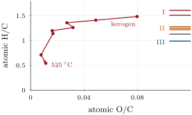
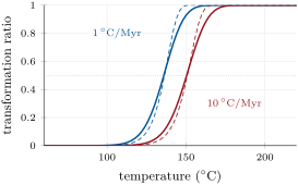
The conversion of kerogen to petroleum is a set of first-order reactions, each obeying the Arrhenius law. In a subsiding basin the temperature of a source rock rises slowly and almost steadily, which makes the following result the core of maturation models.

Proposition 30.2 (First-order reaction at a constant heating rate)

Let a first-order reaction of rate constant $k = A\,e^{-E/RT}$ run in a material heated at the constant rate $\beta = \mathrm{d}T/\mathrm{d}t$ from a temperature $T_0$ at which $k$ is negligible. The fraction left unconverted at the temperature $T$ is

$$x(T) = \exp\Bigl[-\frac{A}{\beta}\int_{T_0}^{T} e^{-E/RT'}\,\mathrm{d}T'\Bigr] \approx \exp\Bigl[-\frac{A R T^2}{\beta E}\,e^{-E/RT}\Bigr] ,\tag{30.1}$$

the approximation holding when $E/RT \gg 1$; the transformation ratio is $1 - x$.

Two consequences follow. Conversion happens over a narrow range of temperature, because $e^{-E/RT}$ changes so fast (exercise 30.11). And slower heating converts at a lower temperature: setting $x = 1/2$, a heating rate ten times faster raises the temperature of half conversion by about $(RT^2/E)\ln 10$. The kinetics of the Green River kerogen, fitted to laboratory pyrolysis, are $A = 9.21 \times 10^{13}\,\mathrm{s}^{-1}$ and $E/R = 26\,800\,\mathrm{K}$ ($E = 223\,\mathrm{kJ}/\mathrm{mol}$); with this single energy, half conversion occurs at $136.4\,{}^{\circ}\mathrm{C}$ for $1\,{}^{\circ}\mathrm{C}/\mathrm{Myr}$ and at $150.9\,{}^{\circ}\mathrm{C}$ for $10\,{}^{\circ}\mathrm{C}/\mathrm{Myr}$, a shift of $14.5\,{}^{\circ}\mathrm{C}$ against $6.26 \times \ln 10 = 14.4\,\mathrm{K}$ predicted. Heated at $10\,\mathrm{K}$ per minute, the same kerogen converts near $450\,{}^{\circ}\mathrm{C}$ (exercise 30.6): time stands in for temperature, which is why kinetics are measured by pyrolysis at about 250 to $600\,{}^{\circ}\mathrm{C}$, and why extrapolating them across twelve orders of magnitude in heating rate leaves the predicted depth of the oil window uncertain.

A real kerogen holds bonds of many strengths, so its kinetics are a distribution of activation energies, each fraction obeying the proposition; for the Green River kerogen the distribution is normal, with a standard deviation $\sigma/R = 481\,\mathrm{K}$. The distribution spreads the conversion, as the right of the figure shows: at $150\,{}^{\circ}\mathrm{C}$ the kerogen heated at $1\,{}^{\circ}\mathrm{C}/\mathrm{Myr}$ is $93\,\%$ converted, the one heated ten times faster $48\,\%$.

Definition 30.3 (Vitrinite reflectance, time–temperature index)

Vitrinite reflectance, $R_o$, is the percentage of incident light reflected by polished grains of vitrinite, an organic component of coal and of kerogen, measured under a microscope; it rises irreversibly with heating and records the highest thermal maturity a rock has reached. The time–temperature index (TTI) of Lopatin is the sum $\sum_n \Delta t_n\,2^n$ over the intervals of $10\,{}^{\circ}\mathrm{C}$ that a rock has passed through, $\Delta t_n$ being the time in millions of years spent in the interval numbered $n$, with $n = 0$ for 100 to $110\,{}^{\circ}\mathrm{C}$, $n = 1$ for 110 to $120\,{}^{\circ}\mathrm{C}$, $n = -1$ for 90 to $100\,{}^{\circ}\mathrm{C}$, and so on.

On the reflectance scale, oil generation from type I and II kerogens begins near $R_o = 0.60\,\%$; above 1.20 to $1.30\,\%$ oil is unstable and breaks down to methane; type III begins to yield methane near $0.73\,\%$, and gas generation goes on up to about $4.8\,\%$. Models compute $R_o$ like a kerogen: the Easy%Ro model treats vitrinite as twenty parallel first-order reactions with $A = 10^{13}\,\mathrm{s}^{-1}$ and energies from 34 to $72\,\mathrm{kcal}/\mathrm{mol}$ (142 to $301\,\mathrm{kJ}/\mathrm{mol}$), and maps their converted fraction $F$, at most 0.85, to $R_o = \exp(-1.6 + 3.7F)$, which runs from 0.20 to $4.7\,\%$.

Reflectance is computed the same way along every horizon of a basin. In the invented basin of the figure below, sediment accumulated at $100\,\mathrm{m}$ per million years from 100 to $70\,\mathrm{Ma}$, then at $35\,\mathrm{m}$ per million years, under a surface at $10\,{}^{\circ}\mathrm{C}$ and a steady gradient of $30\,{}^{\circ}\mathrm{C}/\mathrm{km}$. Its oldest horizon reached $R_o = 0.6\,\%$ at $67.6\,\mathrm{Ma}$, at $3080\,\mathrm{m}$ and $102\,{}^{\circ}\mathrm{C}$, and $1.3\,\%$ at $11.6\,\mathrm{Ma}$, at $5040\,\mathrm{m}$ and $161\,{}^{\circ}\mathrm{C}$; it now lies at $5450\,\mathrm{m}$ and $173.5\,{}^{\circ}\mathrm{C}$, at $R_o = 1.54\,\%$. Because the geotherm is steady, the reflectance fronts run almost along isotherms, the onset of oil generation near $100\,{}^{\circ}\mathrm{C}$, within the 60 to $120\,{}^{\circ}\mathrm{C}$ of the school volumes.

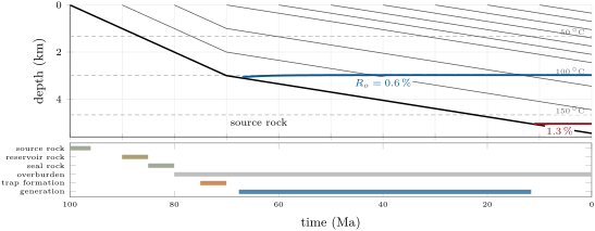
The TTI is older and cruder. It assumes that maturation doubles its rate for every $10\,{}^{\circ}\mathrm{C}$, as an Arrhenius law with $E \approx 82\,\mathrm{kJ}/\mathrm{mol}$ does near $100\,{}^{\circ}\mathrm{C}$ (exercise 30.5); on its scale Waples placed the onset of oil generation at a TTI of 15, its peak at 75 and its end at 160.

Method 30.4 (Computing a time–temperature index)

The data are the burial history of the source rock and the geotherm, assumed steady.

1. Temperature path. Convert depth to temperature at each time: surface temperature plus gradient times depth.
2. Times in the intervals. Find the time $\Delta t_n$ spent in each interval of $10\,{}^{\circ}\mathrm{C}$; where the heating rate $\beta$ is constant, $\Delta t_n = 10\,{}^{\circ}\mathrm{C}/\beta$.
3. Sum. Add the products $\Delta t_n\,2^n$ in order of time; the onset, peak and end of oil generation are reached when the running sum passes 15, 75 and 160.

Basin models express conversion as a transformation ratio: the fraction of the original hydrocarbon potential of a source rock already converted. In one model of a Californian basin, expulsion from the source rock was taken to begin at a ratio of $10\,\%$, to peak at $50\,\%$ and to end at $95\,\%$. The expelled oil, lighter than water, migrates upward into permeable reservoir rocks, and is held where a seal closes a trap.

Proposition 30.5 (Oil in place)

Let a trap have area $A$ and a reservoir of net thickness $h$, porosity $\phi$ and water saturation $S_w$, and let $B_o$ be the formation volume factor of its oil, the ratio of the volume a quantity of oil occupies in the reservoir to its volume at the surface. The stock tank oil initially in place, the oil volume measured at the surface, is

$$\mathrm{STOIIP} = \frac{A\,h\,\phi\,(1 - S_w)}{B_o} .\tag{30.2}$$

Definition 30.6 (Recovery factor)

The recovery factor of a reservoir is the fraction of the oil (or gas) initially in place that is produced over its life.

Primary production and secondary recovery by water injection together typically recover 30 to $40\,\%$ of the oil in place; injecting carbon dioxide recovers 10 to $15\,\%$ more. A trap of $10\,\mathrm{km}^{2}$ with $30\,\mathrm{m}$ of net reservoir, porosity 0.20, oil saturation 0.70 and $B_o = 1.2$ holds $3.5 \times 10^{7}\,\mathrm{m}^{3}$ of stock-tank oil, of which 1.05 to $1.4 \times 10^{7}\,\mathrm{m}^{3}$ would be produced.

30.2 Unconventional resources

Definition 30.7 (Unconventional reservoir)

An unconventional reservoir is a rock of such low permeability that the oil or gas held in its microscopic pores cannot flow to a well at an economic rate without artificial stimulation; it is produced through wells drilled horizontally along it and fractured hydraulically. Shale oil and shale gas are held in the source rock itself, tight gas in low-permeability sandstones and carbonates.

An unconventional play is thus a source rock, or a rock beside it, that kept part of what it generated. Which product it holds follows from its maturity: a shale in the oil window holds oil, one past $R_o \approx 1.3\,\%$ gas. Large-scale production of shale gas began around 2000 in the Barnett Shale of Texas, and most of the growth of United States gas production since 2005 has come from horizontal drilling and hydraulic fracturing in shale, sandstone, carbonate and other tight formations; gas is also produced from coal beds.

30.3 Geothermal energy

Definition 30.8 (Geothermal system, heat in place, enthalpy classes, EGS)

A geothermal system is a volume of the crust where heat, permeability and water come together so that hot water or steam can be produced from wells. The heat in place of a reservoir is the heat it would give up in cooling from its temperature to a reference temperature. A high-enthalpy resource is a geothermal system above about $150\,{}^{\circ}\mathrm{C}$; a low-enthalpy resource one below about $90\,{}^{\circ}\mathrm{C}$; between the two the resource is called moderate. All three suit direct use of the heat, but generally only the moderate and high classes can generate electricity. An enhanced geothermal system (EGS) is a body of hot rock of low natural permeability in which permeability is created by engineering, so that water can be circulated through it and its heat recovered.

Proposition 30.9 (Heat in place and recoverable power)

A reservoir of volume $V$, mean temperature $T_R$ and volumetric heat capacity $C$ (rock and pore fluid together) holds, above the reference temperature $T_0$, the heat

$$q_R = C\,V\,(T_R - T_0) .\tag{30.3}$$

If a fraction $R_g$ of it reaches the wellheads over a production time $\tau$, the mean thermal power produced is $P = R_g\,q_R/\tau$.

Resource assessments use this volume method with a reference of $15\,{}^{\circ}\mathrm{C}$. The recovery factor $R_g$ is the uncertain part: early assessments took 0.25, between 0 and 0.5; production from fractured reservoirs points to about 0.1, between 0.05 and 0.2. With $C = 2.5\,\mathrm{MJ}\,\mathrm{m}^{-3}\,\mathrm{K}^{-1}$ (rock matrices hold 2 to $3\,\mathrm{MJ}\,\mathrm{m}^{-3}\,\mathrm{K}^{-1}$), a reservoir of $3 \times 4 \times 1\,\mathrm{km}$ at $220\,{}^{\circ}\mathrm{C}$ holds $6.15 \times 10^{18}\,\mathrm{J}$; with $R_g = 0.1$ over 30 years it yields a mean thermal power of $650\,\mathrm{MW}$. Conventional fields generate 10 to $20\,\mathrm{MW}$ of electricity per square kilometre of field.

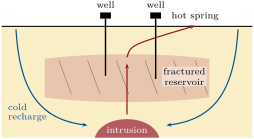
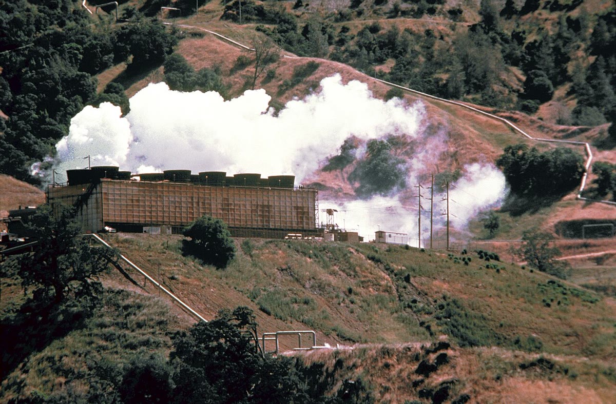
Natural geothermal systems need permeability as much as heat. Most of the major ones lie near the edges of the tectonic plates, among volcanoes, fumaroles, hot springs and geysers, and their permeability is typically that of fractures opened by active faulting: groundwater heated at depth rises through them, and wells tap the fractured reservoir, as in the section below. An EGS needs no natural reservoir: its wells, drilled to about $5\,\mathrm{km}$, reach hot rock whose permeability is engineered, and a 2008 assessment of the United States put its provisional potential at $517\,800\,\mathrm{MW}$ of electricity, against $9057\,\mathrm{MW}$ from identified conventional systems.

Definition 30.10 (Induced seismicity)

Induced seismicity is earthquake activity caused by human operations that change the stress or the pore-fluid pressure in the crust, most often the injection of fluid into the ground.

The mechanism is the Coulomb criterion with pore-fluid pressure: a fault slips when the shear stress reaches $\mu(\sigma_n - p)$, so raising $p$ brings a fault that is already stressed toward failure without any change of the tectonic load. In the 1960s, waste fluid injected into fractured Precambrian basement beneath the Rocky Mountain Arsenal near Denver, at depths of 3.7 to $7.0\,\mathrm{km}$, triggered earthquakes; they were confined to the part of the reservoir where the pressure had risen by more than $32\,\mathrm{bar}$ ($3.2\,\mathrm{MPa}$). The steep rise in the earthquakes of Oklahoma has been attributed to the disposal of wastewater: four high-volume wells could account for a fifth of the seismicity of the central United States, triggering earthquakes more than $30\,\mathrm{km}$ away. Stimulating an EGS reservoir raises the pore pressure in the same way, by design.

30.4 Uranium

Two ore-deposit types illustrate how uranium is concentrated: one at an ancient unconformity, the other in sandstone.

Definition 30.11 (Unconformity-related and roll-front uranium deposits)

An unconformity-related uranium deposit is a body of pitchblende and uraninite filling fractures and breccias in metamorphosed carbonaceous pelites and in the quartz arenites above them, below, above or across an unconformity between Early and Middle Proterozoic rocks in an intracratonic basin. A roll-front uranium deposit is a crescent-shaped body of uranium minerals that cuts across the bedding of a feldspathic or tuffaceous sandstone at the boundary between oxidized and reduced ground, where uranium was deposited in a locally reduced environment, among pyrite.

The unconformity deposits are hosted by rocks of 1800 to $1200\,\mathrm{Ma}$, the metamorphosed pelites below the unconformity and the unmetamorphosed sandstones above it; their host rocks are chloritized, and the graphitic schists that accompany many of them are strong electrical conductors, a target for electromagnetic surveys. Key Lake, Cluff Lake and Rabbit Lake in Saskatchewan and Jabiluka and Ranger in northern Australia are examples. The roll fronts are younger, mostly Tertiary: in sandstones fed by felsic volcanic ash or granite, oxidized iron minerals lie up-dip of the front and reduced ones down-dip, as in the basins of Wyoming and the Texas Gulf Coast.

Proposition 30.12 (Uranium-235 in the past)

Let $r_0$ be today’s atomic ratio $^{235}$U/$^{238}$U and $\lambda_5$, $\lambda_8$ the decay constants of the two isotopes. A time $t$ ago the ratio was

$$r(t) = r_0\,e^{(\lambda_5 - \lambda_8)\,t} ,\tag{30.4}$$

and $^{235}$U made up a fraction $r/(1 + r)$ of the atoms of uranium, neglecting the trace of $^{234}$U.

With $\lambda_5 = 9.8485 \times 10^{-10}\,\mathrm{yr}^{-1}$, $\lambda_8 = 1.551\,25 \times 10^{-10}\,\mathrm{yr}^{-1}$ and today’s abundances $0.7204\,\%$ and $99.2742\,\%$, $r_0 = 0.0072567$; $2.0\,\mathrm{Ga}$ ago $r = 0.0381$ and natural uranium held $3.67\,\%$ of $^{235}$U, five times today’s share.

History — A reactor two billion years old

In 1972, French scientists measuring uranium ore found small but significant deficits of $^{235}$U, which they traced to the Oklo mine in Gabon. There, pods of rock held up to $65\,\%$ uranium with as little as half the normal share of $^{235}$U, and neodymium depleted in its primordial isotope $^{142}$Nd but enriched in the isotopes 143 to 150 that fission produces: chain reactions had run in the ore about two billion years ago, at about $300\,\mathrm{bar}$ and 400 to $500\,{}^{\circ}\mathrm{C}$. Sixteen such natural reactors are known at Oklo and nearby Bangombé, the only two deposits in the world where they have been found; organic matter had helped concentrate the uranium, and the uranium oxide has held most of the actinides and of the non-volatile fission products in place ever since.

30.5 Geological storage of carbon dioxide

Definition 30.13 (Geological $\ce{CO2}$ storage, trapping mechanisms, storage efficiency factor)

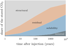
Geological $\ce{CO2}$ storage is the injection of carbon dioxide into porous rock formations deep underground, depleted oil and gas reservoirs, deep saline formations or coal beds, for retention over long times. The $\ce{CO2}$ trapping mechanisms that retain it are structural (and stratigraphic) trapping below a seal; residual trapping, as an immobile phase held in the pores by capillary forces; solubility trapping, by dissolution in the formation water; mineral trapping, by reaction with minerals into carbonates; and, in coal and shale, adsorption onto organic matter. The storage efficiency factor $E$ of a formation is the fraction of its pore volume that the injected $\ce{CO2}$ can be expected to fill.

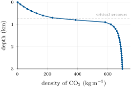
Carbon dioxide is a gas at the surface, but its critical point lies at $31.0\,{}^{\circ}\mathrm{C}$ and $7.38\,\mathrm{MPa}$. Along a geotherm of $25\,{}^{\circ}\mathrm{C}/\mathrm{km}$ from $15\,{}^{\circ}\mathrm{C}$ under hydrostatic pressure, the temperature passes the critical value at $641\,\mathrm{m}$ and the pressure at $742\,\mathrm{m}$; the density of pure $\ce{CO2}$ jumps from $234\,\mathrm{kg}\,\mathrm{m}^{-3}$ at $700\,\mathrm{m}$ to $583\,\mathrm{kg}\,\mathrm{m}^{-3}$ at $900\,\mathrm{m}$, then levels off near 670 to $700\,\mathrm{kg}\,\mathrm{m}^{-3}$ below $1.5\,\mathrm{km}$. A tonne occupies $534\,\mathrm{m}^{3}$ at the surface and $1.6\,\mathrm{m}^{3}$ at $1000\,\mathrm{m}$, 330 times less; this is why storage assessments consider only formations deeper than $800\,\mathrm{m}$.

Proposition 30.14 (Storage capacity of a formation)

A formation of area $A$, thickness $h$ and porosity $\phi$, in which $\ce{CO2}$ has the density $\rho$ and the storage efficiency factor is $E$, can store the mass

$$M = A\,h\,\phi\,\rho\,E .\tag{30.5}$$

For a depleted oil field that has produced a stock-tank volume $N_p$, replacing the produced oil volume for volume gives $M = \rho\,N_p\,B_o$.

For deep saline formations, simulations give $E$ between 1 and $4\,\%$ of the pore volume over a 15 to 85 per cent confidence range, with a median near $2\,\%$: most of the pore space is never reached, or keeps its water. A formation of $1000\,\mathrm{km}^{2}$, $50\,\mathrm{m}$ thick and of porosity 0.20 at $2000\,\mathrm{m}$ ($\rho = 686\,\mathrm{kg}\,\mathrm{m}^{-3}$) stores $137\,\mathrm{Mt}$ at $E = 2\,\%$.

Once injected, the $\ce{CO2}$ rises under the seal and spreads. Behind the migrating plume, capillary forces hold residual saturations that may reach 15 to $25\,\%$ of the pore space; dissolution takes up 20 to $60\,\mathrm{kg}$ of $\ce{CO2}$ per cubic metre of formation water, and in slowly flowing formations up to $30\,\%$ of the injected $\ce{CO2}$ dissolves within tens of years. Solubility trapping dominates over tens to hundreds of years, ionic forms over hundreds to thousands, mineral trapping over thousands to millions: reactions with carbonate minerals take days, with silicates hundreds to thousands of years. The storage becomes more secure as it ages, and at well-chosen and well-managed sites the retention of $99\,\%$ or more of the $\ce{CO2}$ over 1000 years was judged likely.

Figures as of 2005

At Sleipner, in the North Sea about $250\,\mathrm{km}$ off Norway, the $\ce{CO2}$ separated from the natural gas of the field, about $9\,\%$ of it, has been injected since October 1996 into the Utsira formation, an unconsolidated saline sandstone 800 to $1000\,\mathrm{m}$ below the sea floor, at about $1\,\mathrm{Mt}$ a year. By early 2005 more than $7\,\mathrm{Mt}$ had been stored, of the $20\,\mathrm{Mt}$ planned over the project’s life. Repeated seismic surveys image the plume, whose footprint was then about $5\,\mathrm{km}^{2}$, and show that the caprock above it seals it.

In the field — Reading a well while it is drilled

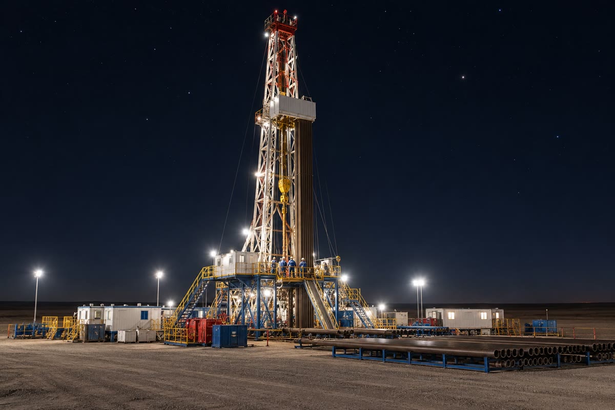
When a section of a well is finished, geophysicists lower tools on a cable and record against depth the properties of the rocks around the hole. One records their natural radioactivity, low in sandstone and higher in shale; another their bulk density, from which the porosity follows as (grain density $-$ bulk density)/(grain density $-$ fluid density), with $2.65\,\mathrm{g}/\mathrm{cm}^{3}$ for quartz grains and about $1\,\mathrm{g}/\mathrm{cm}^{3}$ for the water. Read together, these borehole logs give the net reservoir thickness and the porosity that enter the volumetric formulas of this chapter.

Exercises

Data for the exercises, unless stated otherwise: $R = 8.314\,\mathrm{J}\,\mathrm{mol}^{-1}\,\mathrm{K}^{-1}$; one million years is $3.156 \times 10^{13}\,\mathrm{s}$; Green River kerogen $A = 9.21 \times 10^{13}\,\mathrm{s}^{-1}$, $E/R = 26\,800\,\mathrm{K}$; atomic masses C 12.011, H 1.008, O 15.999; density of $\ce{CO2}$ along the profile of the figure: $1.872\,\mathrm{kg}\,\mathrm{m}^{-3}$ at the surface, 583 at $900\,\mathrm{m}$, 621 at $1000\,\mathrm{m}$, 686 at $2000\,\mathrm{m}$. Round to three significant figures.

Exercise 30.1 ★

(a) Four immature kerogens have atomic H/C of 1.58, 0.95, 1.24 and 1.12. Assign each a type and say which would yield mainly gas. (b) Check the ratios H/C and O/C of the formula C$_{100}$H$_{150}$N$_3$O$_8$S. (c) Find them from the mass composition C $77.4\,\%$, H $9.8\,\%$, O $8.2\,\%$.

Solution

Solution of Exercise 30.1.

(a) 1.58: type I; 0.95: type III; 1.24: type II; 1.12: mixed type II/III. The type III kerogen, at 0.95, yields mainly gas. (b) H/C $= 150/100 = 1.50$, O/C $= 8/100 = 0.08$. (c) Per $100\,\mathrm{g}$: $77.4/12.011 = 6.444\,\mathrm{mol}$ C, $9.8/1.008 = 9.722\,\mathrm{mol}$ H, $8.2/15.999 = 0.513\,\mathrm{mol}$ O; H/C $= 1.51$ and O/C $= 0.0795$, in agreement with the formula.

Exercise 30.2 ★

(a) Five samples of a type II source rock have $R_o$ = 0.45, 0.68, 1.1, 1.6 and $2.5\,\%$. Describe the state of each with respect to oil and gas. (b) Is a type III kerogen at $R_o = 0.68\,\%$ generating methane? (c) Which converted fraction $F$ of Easy%Ro corresponds to $R_o = 0.6$ and $1.3\,\%$?

Solution

Solution of Exercise 30.2.

(a) 0.45: immature, below the onset at $0.60\,\%$; 0.68: generating oil; 1.1: still in the oil window, near its end; 1.6: past 1.20–$1.30\,\%$, so oil breaks down to methane and the rock yields gas; 2.5: gas only, generation continuing up to about $4.8\,\%$. (b) No: methane generation from type III begins near $0.73\,\%$. (c) $F = (\ln R_o + 1.6)/3.7$: $(-0.511 + 1.6)/3.7 = 0.294$ and $(0.262 + 1.6)/3.7 = 0.503$.

Exercise 30.3 ★

A trap covers $6\,\mathrm{km}^{2}$; its reservoir has $25\,\mathrm{m}$ of net thickness, porosity 0.18 and water saturation 0.30, and $B_o = 1.25$. (a) Find the oil volume in the reservoir and the STOIIP. (b) Find the volume produced for recovery factors of 0.30 and 0.40.

Solution

Solution of Exercise 30.3.

(a) In the reservoir, $6 \times 10^6 \times 25 \times 0.18 \times 0.70 = 1.89 \times 10^{7}\,\mathrm{m}^{3}$; $\mathrm{STOIIP} = 1.89 \times 10^7/1.25 = 1.51 \times 10^{7}\,\mathrm{m}^{3}$. (b) $0.30 \times 1.512 \times 10^7 = 4.54 \times 10^{6}\,\mathrm{m}^{3}$ and $0.40 \times 1.512 \times 10^7 = 6.05 \times 10^{6}\,\mathrm{m}^{3}$.

Exercise 30.4 ★

A sandstone aquifer $200\,\mathrm{m}$ thick under $10\,\mathrm{km}^{2}$ is at $75\,{}^{\circ}\mathrm{C}$. (a) Find its heat in place above $15\,{}^{\circ}\mathrm{C}$, with $C = 2.5\,\mathrm{MJ}\,\mathrm{m}^{-3}\,\mathrm{K}^{-1}$. (b) To which enthalpy class does it belong? (c) Find the mean thermal power over 30 years for $R_g = 0.25$.

Solution

Solution of Exercise 30.4.

(a) $V = 10^7 \times 200 = 2 \times 10^{9}\,\mathrm{m}^{3}$ and $q_R = 2.5 \times 10^6 \times 2 \times 10^9 \times 60 = 3.0 \times 10^{17}\,\mathrm{J}$. (b) Below $90\,{}^{\circ}\mathrm{C}$: a low-enthalpy resource, for direct use of the heat. (c) $P = 0.25 \times 3.0 \times 10^{17}/(30 \times 3.156 \times 10^{7}\,\mathrm{s}) = 79.2\,\mathrm{MW}$ of heat.

Exercise 30.5 ★★

(a) Find the activation energy for which an Arrhenius rate doubles between 100 and $110\,{}^{\circ}\mathrm{C}$. (b) By what factor does the rate of the Green River reaction grow over the same interval? (c) Which of the two rules gives more weight to the time a rock spent at low temperature, and what does this imply for a TTI computed for a type I source rock?

Solution

Solution of Exercise 30.5.

(a) $k_2/k_1 = \exp[(E/R)(1/T_1 - 1/T_2)] = 2$ with $1/373.15 - 1/383.15 = 6.994 \times 10^{-5}\,\mathrm{K}^{-1}$ gives $E = 8.314 \times \ln 2/(6.994 \times 10^{-5}) = 82.4\,\mathrm{kJ}/\mathrm{mol}$. (b) $\exp(26800 \times 6.994 \times 10^{-5}) = 6.52$. (c) The doubling rule, whose effective energy is lower, gives relatively more weight to the long times spent at low temperature; for a type I kerogen with a high activation energy, the TTI announces generation too early.

Exercise 30.6 ★★

(a) Show from (30.1) that the temperature of half conversion obeys $T = (E/R)\big/\ln\bigl[A T^2/(\beta\,(E/R)\ln 2)\bigr]$, and solve it by iteration for the Green River kerogen heated at $1\,{}^{\circ}\mathrm{C}/\mathrm{Myr}$ and at $10\,\mathrm{K}$ per minute. (b) Compare the difference with the estimate $(RT^2/E)\ln(\beta_2/\beta_1)$ taken at the lower temperature, and explain the discrepancy.

Solution

Solution of Exercise 30.6.

(a) $x = 1/2$ in the approximation gives $(ART^2/\beta E)\,e^{-E/RT} = \ln 2$; taking logarithms, $E/RT = \ln[AT^2/(\beta(E/R)\ln 2)]$, and the stated form follows. Starting from any guess near $400\,\mathrm{K}$ and iterating with $\beta$ in kelvins per second: at $1\,{}^{\circ}\mathrm{C}/\mathrm{Myr}$ ($\beta = 3.169 \times 10^{-14}\,\mathrm{K}/\mathrm{s}$), $T = 409.6\,\mathrm{K}$, $136.4\,{}^{\circ}\mathrm{C}$; at $10\,\mathrm{K}$ per minute ($\beta = 0.1667\,\mathrm{K}/\mathrm{s}$, $5.26 \times 10^{12}$ times faster), $T = 719.0\,\mathrm{K}$, $445.9\,{}^{\circ}\mathrm{C}$. (b) The difference is $309.5\,\mathrm{K}$; the estimate $6.259 \times \ln(5.26 \times 10^{12}) = 6.259 \times 29.29 = 183\,\mathrm{K}$ is far too small, because $RT^2/E$ itself grows with $T$ (to $19.3\,\mathrm{K}$ at $719\,\mathrm{K}$): the linear shift holds only for small changes of rate.

Exercise 30.7 ★★

Using (30.4) and the data of the text: (a) find the share of $^{235}$U in natural uranium $2.0\,\mathrm{Ga}$ and $1.8\,\mathrm{Ga}$ ago; (b) when was it $3.00\,\%$? (c) Oklo ore holds as little as half today’s normal share of $^{235}$U. Ignoring the $^{238}$U consumed, what fraction of the $^{235}$U present at the time of the reactions was fissioned, and why does the later decay not change the answer?

Solution

Solution of Exercise 30.7.

$\lambda_5 - \lambda_8 = 8.297\,25 \times 10^{-10}\,\mathrm{yr}^{-1}$ and $r_0 = 0.7204/99.2742 = 0.0072567$. (a) At $2.0\,\mathrm{Ga}$, $r = 0.0072567\,e^{1.6595} = 0.03814$, share $0.03814/1.03814 = 3.67\,\%$; at $1.8\,\mathrm{Ga}$, $r = 0.03231$, share $3.13\,\%$. (b) $r = 3/97 = 0.030928$ and $t = \ln(0.030928/0.0072567)/(8.29725 \times 10^{-10}) = 1.75\,\mathrm{Ga}$. (c) Both the depleted ore and normal uranium have decayed since by the same factors, so the ratio of their $^{235}$U shares is the same today as just after the reactions: the ore then held half the normal share, so about half of its $^{235}$U had been fissioned.

Exercise 30.8 ★★

(a) Find the volume of $1\,\mathrm{Mt}$ of $\ce{CO2}$ at the surface, at $1000\,\mathrm{m}$ and at $2000\,\mathrm{m}$. (b) At Sleipner more than $7\,\mathrm{Mt}$ had been injected by 2005, at about $900\,\mathrm{m}$, into a plume of footprint $5\,\mathrm{km}^{2}$. Taking a porosity of 0.35 and a $\ce{CO2}$ saturation of 0.30 in the plume, find the volume of rock it occupies and its mean thickness.

Solution

Solution of Exercise 30.8.

(a) $10^9/1.872 = 5.34 \times 10^{8}\,\mathrm{m}^{3}$; $10^9/621.4 = 1.61 \times 10^{6}\,\mathrm{m}^{3}$; $10^9/686.4 = 1.46 \times 10^{6}\,\mathrm{m}^{3}$. (b) $7 \times 10^9/583 = 1.20 \times 10^{7}\,\mathrm{m}^{3}$ of $\ce{CO2}$, filling $0.35 \times 0.30 = 0.105$ of the rock volume: $1.20 \times 10^7/0.105 = 1.14 \times 10^{8}\,\mathrm{m}^{3}$ of rock, a mean thickness of $1.143 \times 10^8/(5 \times 10^6) = 22.9\,\mathrm{m}$.

Exercise 30.9 ★★

A high-enthalpy reservoir measures $3 \times 2 \times 1.5\,\mathrm{km}$ at $250\,{}^{\circ}\mathrm{C}$, with $C = 2.6\,\mathrm{MJ}\,\mathrm{m}^{-3}\,\mathrm{K}^{-1}$. (a) Find its heat in place above $15\,{}^{\circ}\mathrm{C}$. (b) Find the mean thermal power over 30 years for $R_g = 0.1$ and $0.25$. (c) Its field covers $6\,\mathrm{km}^{2}$; at 10 to $20\,\mathrm{MW}$ of electricity per square kilometre, what fraction of the thermal power at $R_g = 0.1$ becomes electricity?

Solution

Solution of Exercise 30.9.

(a) $V = 9 \times 10^{9}\,\mathrm{m}^{3}$ and $q_R = 2.6 \times 10^6 \times 9 \times 10^9 \times 235 = 5.50 \times 10^{18}\,\mathrm{J}$. (b) Over $30 \times 3.156 \times 10^{7}\,\mathrm{s} = 9.47 \times 10^{8}\,\mathrm{s}$: $R_g = 0.1$ gives $581\,\mathrm{MW}$ and $0.25$ gives $1450\,\mathrm{MW}$ of heat. (c) $6 \times (10 \text{ to } 20) = 60$ to $120\,\mathrm{MW}$ of electricity, $60/581 = 0.10$ to $120/581 = 0.21$ of the thermal power: most of the heat is rejected, as in any power plant working with a modest temperature difference.

Exercise 30.10 ★★★

A fault at about $4\,\mathrm{km}$ carries a normal stress of $80\,\mathrm{MPa}$ and a shear stress of $22\,\mathrm{MPa}$; its friction coefficient is 0.6 and the pore pressure is hydrostatic, $39\,\mathrm{MPa}$. (a) Is the fault stable? Find the pore-pressure rise that brings it to failure, in megapascals and in bars, and compare with the Denver threshold. (b) The same if the shear stress is $24\,\mathrm{MPa}$. (c) Explain why earthquakes can be triggered kilometres away from an injection well, and years after injection began.

Solution

Solution of Exercise 30.10.

(a) The strength is $0.6 \times (80 - 39) = 24.6\,\mathrm{MPa} > 22\,\mathrm{MPa}$: stable. Failure needs $0.6\,\Delta p = 24.6 - 22$, $\Delta p = 4.33\,\mathrm{MPa} = 43\,\mathrm{bar}$, of the same order as the $32\,\mathrm{bar}$ that bounded the Denver earthquakes. (b) $(24.6 - 24)/0.6 = 1.0\,\mathrm{MPa} = 10\,\mathrm{bar}$: a fault already close to failure needs only a small rise. (c) Injected fluid raises the pressure in a zone that spreads by diffusion through permeable rock and fault zones, kilometres away over years; wherever it meets a fault already near failure, a modest rise is enough.

Exercise 30.11 ★★★

(a) From the approximation in (30.1), show that at a constant heating rate the transformation ratio rises from $10\,\%$ to $90\,\%$ over a temperature interval $\Delta T \approx \bigl[\ln\ln 10 - \ln\ln(10/9)\bigr]\,RT^2/E$. (b) Evaluate it for the Green River kerogen at $1\,{}^{\circ}\mathrm{C}/\mathrm{Myr}$. (c) Compare with the solid curve of the figure and explain the difference.

Solution

Solution of Exercise 30.11.

(a) Write $x = e^{-u}$ with $u = (ART^2/\beta E)\,e^{-E/RT}$. A transformation ratio of $10\,\%$ means $x = 0.9$, $u = \ln(10/9)$; $90\,\%$ means $u = \ln 10$. As $\mathrm{d}\ln u/\mathrm{d}T = E/RT^2 + 2/T \approx E/RT^2$, $\Delta(\ln u) \approx (E/RT^2)\,\Delta T$, which gives the formula, with $\ln\ln 10 - \ln\ln(10/9) = 0.834 + 2.250 = 3.084$. (b) With $T = 409.6\,\mathrm{K}$, $RT^2/E = 6.26\,\mathrm{K}$ and $\Delta T = 19.3\,\mathrm{K}$; the exact single-energy curve gives $18.6\,\mathrm{K}$, from 125.3 to $143.8\,{}^{\circ}\mathrm{C}$. (c) The solid curve rises from $10\,\%$ near $122\,{}^{\circ}\mathrm{C}$ to $90\,\%$ near $148\,{}^{\circ}\mathrm{C}$, over about $26\,\mathrm{K}$: the spread of activation energies widens the conversion interval.

Exercise 30.12 ★★★

Sleipner is to store $20\,\mathrm{Mt}$ of $\ce{CO2}$. (a) Find the volume of formation water needed to dissolve it all, at 20 and at $60\,\mathrm{kg}\,\mathrm{m}^{-3}$. (b) Find its volume as a free phase at $1000\,\mathrm{m}$. (c) With $E = 2\,\%$, find the pore volume of formation required, and the area of a formation $50\,\mathrm{m}$ thick of porosity 0.30.

Solution

Solution of Exercise 30.12.

(a) $2 \times 10^{10}/20 = 1.0 \times 10^{9}\,\mathrm{m}^{3}$ ($1.0\,\mathrm{km}^{3}$) and $2 \times 10^{10}/60 = 3.3 \times 10^{8}\,\mathrm{m}^{3}$. (b) $2 \times 10^{10}/621.4 = 3.22 \times 10^{7}\,\mathrm{m}^{3}$. (c) $3.22 \times 10^7/0.02 = 1.61 \times 10^{9}\,\mathrm{m}^{3}$ of pores, which with $50 \times 0.30 = 15\,\mathrm{m}$ of pore space per square metre requires $1.61 \times 10^9/15 = 1.07 \times 10^{8}\,\mathrm{m}^{2}$, about $107\,\mathrm{km}^{2}$.

Problem 30.1

Weekend problem — One basin, two uses

In an invented basin, a type I source rock was deposited at $120\,\mathrm{Ma}$ at the surface. Sediment then accumulated at $60\,\mathrm{m}$ per million years until $70\,\mathrm{Ma}$, and at $30\,\mathrm{m}$ per million years since. The surface is at $15\,{}^{\circ}\mathrm{C}$ and the geotherm is steady at $25\,{}^{\circ}\mathrm{C}/\mathrm{km}$. The kerogen has the Green River kinetics of the text (single energy). Its kitchen, the mature part of the source rock, covers $400\,\mathrm{km}^{2}$, is $50\,\mathrm{m}$ thick and of density $2400\,\mathrm{kg}\,\mathrm{m}^{-3}$, and can yield $30\,\mathrm{kg}$ of oil per tonne of rock at full conversion; the oil has a surface density of $850\,\mathrm{kg}\,\mathrm{m}^{-3}$. The oil fills a trap of $12\,\mathrm{km}^{2}$ whose reservoir, centred at $2000\,\mathrm{m}$, has a net thickness of $40\,\mathrm{m}$, porosity 0.22 and water saturation 0.25, with $B_o = 1.30$. Use the data of the exercises; round to three significant figures.

Part I — Burial and the time–temperature index.

1. Find the depth and temperature of the source rock at $70\,\mathrm{Ma}$ and today.
2. Find its heating rate in each phase.
3. Find the time it spent in each interval of $10\,{}^{\circ}\mathrm{C}$, from $15\,{}^{\circ}\mathrm{C}$ to its present temperature.
4. Compute its TTI today (method of the text).
5. When, at what temperature and at what depth did it pass a TTI of 15?
6. The same for 75 and 160.
7. By the TTI, is the source rock still generating oil?

Part II — Conversion by kinetics.

8. Find the rate constant at $90\,{}^{\circ}\mathrm{C}$ and show that less than $0.2\,\%$ of the kerogen can have been converted before $70\,\mathrm{Ma}$.
9. Using (30.1) with the heating rate of the second phase, find the unconverted fraction and the transformation ratio today.
10. Find the temperature of half conversion at this heating rate (exercise 30.6).
11. When was it reached?
12. Compare with the time of peak generation given by the TTI, and explain the difference.
13. Would a type II kerogen with a lower mean activation energy have converted earlier or later?

Part III — Oil generated, in place and recoverable.

14. Taking a transformation ratio of 0.92, find the mass of oil generated in the kitchen.
15. Find its volume at the surface.
16. Find the STOIIP of the trap.
17. What fraction of the oil generated does the trap hold? Keep $1.56 \times 10^{9}\,\mathrm{m}^{3}$ for (15).
18. Find the oil produced for a recovery factor of 0.35.
19. Why is the recovery factor much less than one, and what would injecting $\ce{CO2}$ change?

Part IV — The depleted field as a $\ce{CO2}$ store.

20. Find the temperature and hydrostatic pressure of the reservoir. Is injected $\ce{CO2}$ supercritical there? Read its density on the figure.
21. Keeping $N_p = 2.13 \times 10^{7}\,\mathrm{m}^{3}$, find the reservoir volume freed by production.
22. Express it as a storage efficiency factor of the pore volume of the trap, and compare with saline formations.
23. A saline formation below the field covers $600\,\mathrm{km}^{2}$, is $80\,\mathrm{m}$ thick, of porosity 0.20, with $\ce{CO2}$ at $691\,\mathrm{kg}\,\mathrm{m}^{-3}$. Find its capacity at $E = 2\,\%$.
24. How many years of injection at the Sleipner rate would fill it?
25. With $\rho = 686\,\mathrm{kg}\,\mathrm{m}^{-3}$ and the freed volume rounded to $2.77 \times 10^{7}\,\mathrm{m}^{3}$, find the $\ce{CO2}$ storage capacity of the depleted reservoir, in megatonnes.

Solution

Solution of Problem 30.1.

Part I. 1. At $70\,\mathrm{Ma}$: $50 \times 60 = 3000\,\mathrm{m}$, $15 + 25 \times 3.0 = 90\,{}^{\circ}\mathrm{C}$. Today: $3000 + 70 \times 30 = 5100\,\mathrm{m}$, $142.5\,{}^{\circ}\mathrm{C}$. 2. $60 \times 0.025 = 1.5\,{}^{\circ}\mathrm{C}/\mathrm{Myr}$, then $30 \times 0.025 = 0.75\,{}^{\circ}\mathrm{C}/\mathrm{Myr}$. 3. 15–$20\,{}^{\circ}\mathrm{C}$: $3.33\,\mathrm{Myr}$; each interval from 20 to $90\,{}^{\circ}\mathrm{C}$: $10/1.5 = 6.67\,\mathrm{Myr}$; each from 90 to $140\,{}^{\circ}\mathrm{C}$: $10/0.75 = 13.3\,\mathrm{Myr}$; 140–$142.5\,{}^{\circ}\mathrm{C}$: $3.33\,\mathrm{Myr}$. 4. Interval values $\Delta t_n 2^n$, with running sums: 15–20 ($n = -9$) 0.0065; 20–30 0.026 (0.033); 30–40 0.052 (0.085); 40–50 0.104 (0.189); 50–60 0.208 (0.397); 60–70 0.417 (0.814); 70–80 0.833 (1.65); 80–90 1.67 (3.31); 90–100 6.67 (9.98); 100–110 13.3 (23.3); 110–120 26.7 (50.0); 120–130 53.3 (103); 130–140 107 (210); 140–142.5 ($n = 4$) 53.3: TTI today 263. 5. 15 is passed in the interval 100–$110\,{}^{\circ}\mathrm{C}$, at $100 + 10 \times (15 - 9.98)/13.33 = 103.8\,{}^{\circ}\mathrm{C}$, reached $(103.8 - 90)/0.75 = 18.4\,\mathrm{Myr}$ after $70\,\mathrm{Ma}$: at $51.6\,\mathrm{Ma}$ and $(103.8 - 15)/0.025 = 3550\,\mathrm{m}$. 6. 75: $124.7\,{}^{\circ}\mathrm{C}$, $23.7\,\mathrm{Ma}$, $4390\,\mathrm{m}$. 160: $135.3\,{}^{\circ}\mathrm{C}$, $9.6\,\mathrm{Ma}$, $4810\,\mathrm{m}$. 7. No: at 263 it is past the end of oil generation (160), since about $10\,\mathrm{Ma}$.

Part II. 8. $k = 9.21 \times 10^{13}\,e^{-26800/363.15} = 8.20 \times 10^{-19}\,\mathrm{s}^{-1}$. The rock was below $90\,{}^{\circ}\mathrm{C}$ for the $50\,\mathrm{Myr}$ before $70\,\mathrm{Ma}$, so the converted fraction is less than $k\,t = 8.20 \times 10^{-19} \times 50 \times 3.156 \times 10^{13} = 1.29 \times 10^{-3}$. 9. $\beta = 0.75/(3.156 \times 10^{13}) = 2.376 \times 10^{-14}\,\mathrm{K}/\mathrm{s}$, $T = 415.65\,\mathrm{K}$: $ART^2/(\beta E) = 2.498 \times 10^{28}$ and $e^{-E/RT} = 9.95 \times 10^{-29}$, so $u = 2.486$, $x = 0.0833$ and the transformation ratio is 0.917. 10. $134.7\,{}^{\circ}\mathrm{C}$. 11. $70 - (134.7 - 90)/0.75 = 10.4\,\mathrm{Ma}$. 12. The TTI places peak generation at $23.7\,\mathrm{Ma}$, the kinetics $13\,\mathrm{Myr}$ later, because the doubling rule corresponds to $E \approx 82\,\mathrm{kJ}/\mathrm{mol}$ and weights the low temperatures too much for a kerogen of $223\,\mathrm{kJ}/\mathrm{mol}$ (exercise 30.5). 13. Earlier: a lower energy lowers the temperature of half conversion.

Part III. 14. Rock: $4 \times 10^8 \times 50 \times 2400 = 4.8 \times 10^{13}\,\mathrm{kg}$; potential $0.030 \times 4.8 \times 10^{13} = 1.44 \times 10^{12}\,\mathrm{kg}$; generated $0.92 \times 1.44 \times 10^{12} = 1.32 \times 10^{12}\,\mathrm{kg}$. 15. $1.3248 \times 10^{12}/850 = 1.56 \times 10^{9}\,\mathrm{m}^{3}$. 16. $1.2 \times 10^7 \times 40 \times 0.22 \times 0.75/1.30 = 6.09 \times 10^{7}\,\mathrm{m}^{3}$. 17. $6.09 \times 10^7/1.56 \times 10^9 = 0.039$, $3.9\,\%$: most generated oil stays in the source rock, is lost along the migration paths or escapes to the surface. 18. $0.35 \times 6.09 \times 10^7 = 2.13 \times 10^{7}\,\mathrm{m}^{3}$. 19. About two thirds of the oil stays in the reservoir after primary and secondary recovery; $\ce{CO2}$ injection could recover a further 10 to $15\,\%$ of the oil in place.

Part IV. 20. $15 + 25 \times 2 = 65\,{}^{\circ}\mathrm{C}$ and $0.101 + 1000 \times 9.807 \times 2000/10^6 = 19.7\,\mathrm{MPa}$: both above the critical point ($31.0\,{}^{\circ}\mathrm{C}$, $7.38\,\mathrm{MPa}$), so the $\ce{CO2}$ is supercritical, at about $686\,\mathrm{kg}\,\mathrm{m}^{-3}$. 21. $2.13 \times 10^7 \times 1.30 = 2.77 \times 10^{7}\,\mathrm{m}^{3}$. 22. Pore volume $1.2 \times 10^7 \times 40 \times 0.22 = 1.056 \times 10^{8}\,\mathrm{m}^{3}$, and $E = 2.77 \times 10^7/1.056 \times 10^8 = 0.262$, far above the 1 to $4\,\%$ of saline formations: the produced oil has emptied a known, sealed space. 23. $6 \times 10^8 \times 80 \times 0.20 \times 691 \times 0.02 = 1.33 \times 10^{11}\,\mathrm{kg}$, $133\,\mathrm{Mt}$. 24. At $1\,\mathrm{Mt}$ a year, about 133 years. 25. $M = \rho\,N_p\,B_o = 686 \times 2.77 \times 10^7 = 1.90 \times 10^{10}\,\mathrm{kg}$: the depleted reservoir can store $19.0\,\mathrm{Mt}$ of $\ce{CO2}$.