28Geological Hazards and Risk

A building designed for the ground motion that is exceeded, on average, once in 475 years has a one-in-ten chance of meeting it during a fifty-year life. The two statements are the same number read in two ways, and moving between them is the daily work of hazard science. This chapter builds its tools: the probability of rare events, the hazard curve of a site, the stability of a slope, the speed and the run-up of a tsunami, the frequency of floods, and the physics that sets how much warning each hazard can give.

You already know

From the school volumes: natural hazard, natural disaster and landslide; vulnerability, risk, prevention and the hazard map; tsunami; the return period of a flood, and the rank formula $T = (n + 1)/m$ for a record of $n$ annual peaks. From the Year 1 volume: the Gutenberg–Richter law $\log_{10} N(\geq M) = a - bM$ and its b-value; seismic moment and moment magnitude; pore-fluid pressure, effective stress $\sigma' = \sigma - u$ and the Coulomb failure criterion $\tau = c' + \sigma' \tan\varphi'$. From Chapter 6: pyroclastic density currents, lahars and tephra fall. From the mathematics books: the Poisson and exponential distributions, the normal distribution and its distribution function $\Phi$. From the physics books’ Year 2 volume: the dispersion relation of surface gravity waves, $\omega^2 = gk\tanh(kh)$.

28.1 Hazard, exposure and risk

Definition 28.1 (Geological hazard, exposure, disaster risk)

A geological hazard is a process or phenomenon that originates in the internal processes of the Earth — an earthquake, an eruption, a mass movement such as a landslide or a debris flow — and may cause loss of life, injury, damage or disruption. It is characterised by its location, its intensity or magnitude, and its frequency or probability. The exposure to a hazard is the situation of the people, buildings, infrastructure and other assets located where the hazard can reach, measured by their number or their value. Disaster risk is the potential loss of life, health or assets that could occur in a given period, determined probabilistically from the hazard, the exposure and the vulnerability of what is exposed.

The international terminology classes tsunamis apart: triggered by earthquakes and other geological events, they become an oceanic process and strike as a coastal, water-related hazard. This chapter treats them with the others, because their source is geological.

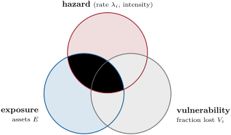
The definition contains a product. If events of intensity $i$ occur at an annual rate $\lambda_i$, if the exposed assets are worth $E$, and if an event of intensity $i$ destroys a fraction $V_i$ of them (the vulnerability, between 0 and 1), the expected annual loss is

often abbreviated to risk = hazard $\times$ exposure $\times$ vulnerability. The risk vanishes when any factor does: a violent volcano on an empty island, a crowded city on a quiet craton, or buildings that resist the shaking. Hazard science measures the first factor; the figure below places it among the three.

28.2 The probability of rare events

Definition 28.2 (Return period)

Let events of a given kind — a flood above a discharge, a ground motion above a level, an earthquake above a magnitude — occur at a mean annual rate $\lambda$. Their return period is $T = 1/\lambda$: the mean interval between two of them, and the inverse of their annual rate, not a timetable.

Definition 28.3 (Exceedance probability)

The exceedance probability of a level in an exposure time $t$ is the probability that the level is equalled or exceeded at least once during $t$.

Proposition 28.4 (Poisson recurrence model)

Suppose that events occur one at a time, independently of one another and of the time elapsed, at a constant mean rate $\lambda = 1/T$. Then the number $N$ of events in a time $t$ follows the Poisson distribution of mean $\lambda t$; the exceedance probability in $t$ is

$$P(t) = 1 - e^{-t/T};\tag{28.2}$$

and the interval between successive events follows the exponential distribution of mean $T$.

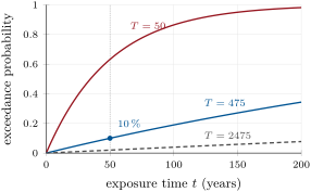
Two consequences are used everywhere. For a probability $p$ in an exposure time $t$, the return period is $T = -t/\ln(1 - p)$: $10\,\%$ in 50 years gives $T = 50/0.10536 = 474.6$ years, the “475-year” motion of building codes, and $2\,\%$ in 50 years gives 2475 years. And when $t \ll T$, $P \approx t/T$: the rate can be read as a probability per year. Over one full return period, by contrast, the probability is $1 - e^{-1} = 63\,\%$, not 1. The figure below (left) draws (28.2) for three return periods.

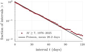
Is the model true? The global catalogue of earthquakes of magnitude at least 7 holds 696 events from 1976 to 2025, 695 intervals with a mean of 26.2 days. If they were a Poisson process, the fraction of intervals longer than $t$ would be $e^{-t/26.2}$, a straight line on a logarithmic axis. The figure below (right) shows that it nearly is: $30.4\,\%$ of the intervals are longer than 30 days, against $31.8\,\%$ for the model, and the standard deviation of the intervals is 1.07 times their mean, against exactly 1. The defect is at short intervals: 36 pairs fall on the same day, aftershocks and doublets that a memoryless process would not cluster. Hazard maps therefore remove the dependent events from a catalogue, declustering it, so that the mainshocks left can be treated as a Poisson process; their rates by magnitude come from the Gutenberg–Richter law.

28.3 Seismic hazard

Definition 28.5 (Probabilistic seismic hazard analysis, ground-motion prediction equation, peak ground acceleration, hazard curve)

The peak ground acceleration (PGA) at a site is the largest absolute horizontal acceleration of the ground during an earthquake, usually expressed as a fraction of $g$. A ground-motion prediction equation (GMPE) gives the probability distribution of a measure of shaking such as the PGA at a site — a median and a scatter — as a function of the magnitude, the distance to the source and the ground conditions. Probabilistic seismic hazard analysis (PSHA) combines all the earthquakes that can affect a site, with their rates and distances, with a GMPE, to give the annual rate at which each level of shaking is exceeded. The curve of that rate against the level is the site’s hazard curve.

The PGA is what a particle of the ground experiences. A building responds to the part of the motion near its own natural period, and codes also map that response, the spectral acceleration; the PGA keeps the reasoning simple and is used here.

Method 28.6 (A probabilistic seismic hazard analysis)

1. Sources. Map the faults and source zones around the site, and the distance $d$ of each to the site.
2. Recurrence. For each source, take the annual rate of earthquakes by magnitude from a Gutenberg–Richter law, truncated at a maximum magnitude $M_{\max}$: $N(\geq m) = 10^{a - bm} - 10^{a - bM_{\max}}$, from a minimum magnitude $M_{\min}$. Cut the range into slices of rate $\nu_j$ around magnitudes $m_j$.
3. Ground motion. From the GMPE, take the median $\mu_j = \log_{10}\mathrm{PGA}$ and the scatter $\sigma$ for each slice; the probability that the PGA exceeds $a$ is $1 - \Phi\bigl((\log_{10} a - \mu_j)/\sigma\bigr)$.
4. Sum. The annual rate of exceedance of $a$ is $\lambda(a) = \sum_j \nu_j \bigl[1 - \Phi\bigl((\log_{10} a - \mu_j)/\sigma\bigr)\bigr]$, summed over all sources.
5. Read. The PGA with a probability $p$ of exceedance in $t$ years is the level where $\lambda(a) = -\ln(1 - p)/t$: $2.107 \times 10^{-3}$ per year for $10\,\%$ in 50 years.

The GMPE used in this chapter is that of Boore, Joyner and Fumal, fitted to 271 recordings of 20 earthquakes in western North America: for a random horizontal component, in units of $g$,

with $M$ the moment magnitude, $d$ the distance in kilometres to the surface projection of the rupture, and a scatter $\sigma = 0.230$ about the median. It holds for $5.0 \leq M \leq 7.7$ and $d \leq 100\,\mathrm{km}$. The constant $5.57\,\mathrm{km}$ is a fictitious depth fitted by the regression, which keeps the motion finite above the source. A magnitude 6 at $15\,\mathrm{km}$ gives a median of $0.091\,\mathrm{g}$, a magnitude 7.5 $0.200\,\mathrm{g}$; one standard deviation multiplies or divides the median by $10^{0.230} = 1.70$.

The terms $G_B$ and $G_C$ carry the site effect. Sites are classed by the mean shear-wave speed of their upper $30\,\mathrm{m}$: class A above $750\,\mathrm{m}\,\mathrm{s}^{-1}$ ($G_B = G_C = 0$), class B from 360 to $750\,\mathrm{m}\,\mathrm{s}^{-1}$ ($G_B = 1$) and class C from 180 to $360\,\mathrm{m}\,\mathrm{s}^{-1}$ ($G_C = 1$). Soft ground multiplies the rock motion by $10^{0.162} = 1.45$ in class B and $10^{0.251} = 1.78$ in class C: a wave entering slower material slows, shortens and grows in amplitude, and a soft layer or a sediment-filled basin can resonate and trap it.

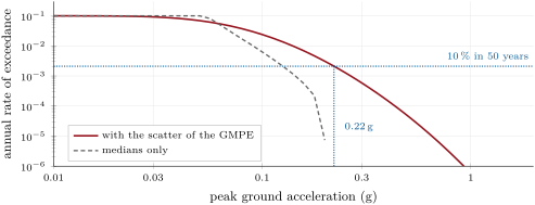
The figure below applies the method to a single source zone $15\,\mathrm{km}$ from a rock site, with $a = 4.0$, $b = 1.0$, $M_{\min} = 5$ and $M_{\max} = 7.5$: about 0.1 earthquake of magnitude 5 or more per year. At small PGA the curve tends to that rate, since every earthquake exceeds a weak level. The $10\,\%$-in-50-years PGA is $0.22\,\mathrm{g}$. Had each earthquake produced exactly its median, the same rate would be reached at $0.13\,\mathrm{g}$, and no level above the median of the largest earthquake, $0.20\,\mathrm{g}$, could ever be exceeded. The scatter dominates the rare levels: the 475-year motion comes largely from moderate earthquakes that shake harder than their median.

28.4 Volcanic hazard

A volcano threatens through several processes at once, each with its own reach: tephra falls far downwind, pyroclastic density currents and lahars follow valleys, lava flows advance slowly (Chapter 6). Its hazard map draws a zone for each, from the deposits of past eruptions and from models of flow and fall. The probabilities are built differently from those of earthquakes, because an awakening volcano is not a stationary process. An event tree leads from unrest to outcomes through branches, each from a necessary prior event to a more specific outcome — unrest, magmatic or not; eruption or not; explosive or effusive; a pyroclastic flow reaching a given valley or not. The probability of an outcome is the product of the conditional probabilities along its branch. With $M$ a magmatic unrest, $E$ an eruption, $X$ an explosive eruption and $V$ a flow in the valley,

each factor estimated from the volcano’s past, from comparable volcanoes or from models, and revised with Bayes’ theorem as new monitoring data arrive (Exercise 28.8).

28.5 Landslides

A slope stands as long as the strength of its material, along any surface on which it could slide, exceeds the stress that gravity applies there. The strength is the Coulomb criterion of the Year 1 volume, written in effective stress: water in the pores carries part of the normal load and lowers the friction.

Definition 28.7 (Factor of safety, debris flow)

The factor of safety $F$ of a slope along a potential slip surface is the ratio of the shear strength available on the surface to the shear stress required for equilibrium. The slope is stable for $F > 1$ and fails when $F$ falls to 1. A debris flow is a rapid flow of water-saturated mud, sand, gravel, boulders and wood that moves down a channel as one dense mass, the grains carrying much of its weight, and spreads on the fan at the mouth of the channel.

Proposition 28.8 (Infinite slope)

A layer of soil of unit weight $\gamma$ and thickness $z$, measured vertically, rests on a slip surface parallel to the ground at an angle $\beta$; its strength is $c'$ and $\varphi'$, and the pore pressure on the surface is $u = r_u \gamma z$. If the layer is long enough for its ends to be neglected,

$$F = \frac{c' + \gamma z\,(\cos^2\beta - r_u)\tan\varphi'}{\gamma z \sin\beta\cos\beta}.\tag{28.4}$$

For a dry, cohesionless layer, $F = \tan\varphi'/\tan\beta$: it stands up to $\beta = \varphi'$.

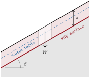
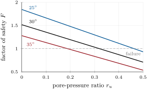
Equation (28.4) names the two common triggers. Rain raises the water table and with it $r_u$; $F$ falls linearly with $r_u$, so that a slope that is safe when dry fails when wet: in the figure above, the $35{}^{\circ}$ slope fails at $r_u = 0.19$, the $25{}^{\circ}$ slope only at 0.46. Shaking adds a horizontal force: if it is represented by $kW$, $k$ a fraction of $g$, the numerator loses $\gamma z k \sin\beta\cos\beta\tan\varphi'$ and the denominator gains $\gamma z k\cos^2\beta$ — a pseudo-static analysis, admitted here, which replaces a brief shaking by a steady force. The cohesion term, $c'/(\gamma z\sin\beta\cos\beta)$, falls as the layer thickens, so cohesion protects thin soils more than deep ones.

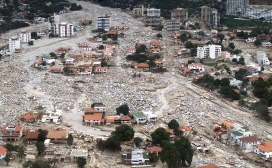
In December 1999 a storm of three days dropped $911\,\mathrm{mm}$ of rain at Maiquetia, on the coast north of Caracas. Thousands of shallow landslides started on the slopes of the Sierra de Avila, on slopes from $30{}^{\circ}$ to more than $60{}^{\circ}$, $42{}^{\circ}$ on average. In the channels they merged into debris flows, which moved at 3 to $14\,\mathrm{m}\,\mathrm{s}^{-1}$ by the superelevation of their surface in bends, and carried boulders up to $11\,\mathrm{m}$ long. On the fan of Caraballeda, shown below, they left up to $6\,\mathrm{m}$ of bouldery debris, about 1.8 million cubic metres. The number of dead is generally given as about $30\,000$.

28.6 Tsunamis

A tsunami raised by the sudden uplift of the sea floor has a wavelength of tens to hundreds of kilometres, far more than the depth of the ocean. It is a long wave, and its speed depends only on the depth.

Proposition 28.9 (Long waves)

A surface gravity wave whose wavelength is much larger than the water depth $h$ travels at $c = \sqrt{gh}$, whatever its wavelength. Where it moves slowly into shallower water without reflecting or breaking, its amplitude $A$ grows as $h^{-1/4}$.

Over $4000\,\mathrm{m}$ of water a tsunami travels at $198\,\mathrm{m}\,\mathrm{s}^{-1}$, $713\,\mathrm{km}/\mathrm{h}$; over $5000\,\mathrm{m}$, $797\,\mathrm{km}/\mathrm{h}$, the “more than 800 km/h” quoted by the warning services. Near the shore, in $10\,\mathrm{m}$ of water, it slows to $36\,\mathrm{km}/\mathrm{h}$; its front is caught up by the water behind, the wave shortens and steepens, and its height grows.

Definition 28.10 (Tsunami run-up)

The tsunami run-up at a point of the coast is the height, above the sea level at the time, of the highest ground that the water reaches inland there. The horizontal distance from the shoreline to that point is the inundation distance.

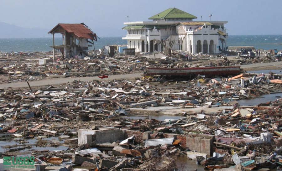
Survey teams measure run-ups from water marks, debris lines and damage after each tsunami. The global tsunami database holds $2177$ run-up observations for the Indian Ocean tsunami of 26 December 2004, raised by a magnitude 9.1 earthquake off Sumatra, with a maximum water height of $50.9\,\mathrm{m}$, and $6429$ for the tsunami of 11 March 2011 off Honshu, also of magnitude 9.1, with a maximum of $39.3\,\mathrm{m}$. The two killed $227\,899$ and $18\,423$ people. In Banda Aceh, the water reached the middle of the second floor of the mosque below.

28.7 Floods

Definition 28.11 (Flood frequency curve)

The flood frequency curve of a river at a gauging station is the curve of the annual peak discharge against its return period, or its annual exceedance probability, built from the station’s record of annual peaks and usually extended by a fitted probability law.

The rank formula of the school volumes places the points of the curve. It has a reason.

Proposition 28.12 (Weibull plotting position)

Let $n$ annual peaks be independent and drawn from the same continuous distribution, and let $G(x)$ be the probability that a year’s peak exceeds $x$. The peak of rank $m$, counted from the largest, has an expected exceedance probability $m/(n + 1)$, so that it is plotted at $T = (n + 1)/m$.

The largest peak of a 30-year record is thus plotted at 31 years, and nothing in the record fixes the 100-year flood. To reach it, the peaks are fitted with a law of extremes, often Gumbel’s, $\Pr(\text{peak} \leq x) = \exp\bigl(-e^{-(x - u)/\alpha}\bigr)$, whose $T$-year flood is $x_T = u - \alpha\ln\bigl(-\ln(1 - 1/T)\bigr)$: a straight line against $-\ln(-\ln(1 - 1/T))$, extrapolated beyond the record at a risk that grows with the distance.

28.8 Monitoring and early warning

Definition 28.13 (Early warning system)

An early warning system is an integrated system of hazard monitoring, forecasting, risk assessment, communication and preparedness that enables timely action before a hazardous event. It joins four elements: knowledge of the risk; detection, monitoring and forecasting of the hazard; the dissemination of warnings; and the preparedness to respond.

Physics sets how much time each warning can give. Seismic waves cannot be outrun, but the damaging S waves travel at about $3.2\,\mathrm{km}\,\mathrm{s}^{-1}$ in the upper crust, against $5.8\,\mathrm{km}\,\mathrm{s}^{-1}$ for the P waves: an alert computed from the first P waves recorded near the epicentre reaches a city before the S waves, by $d(1/3.2 - 1/5.8) = 0.14\,\mathrm{s}$ per kilometre of distance $d$, less the time to detect and compute. A city $100\,\mathrm{km}$ away gains at most $14\,\mathrm{s}$; near the source a blind zone gets none (Exercise 28.12). A tsunami crossing $100\,\mathrm{km}$ of sea $2000\,\mathrm{m}$ deep takes 12 minutes; across an ocean it takes hours. In 2011, the Japanese warning was issued about three minutes after the earthquake, but on a magnitude estimated too low, because the instruments saturated; it was updated with data from an offshore GPS buoy about 28 minutes later. Deep-ocean pressure recorders, which convert the pressure on the sea floor every 15 seconds into a sea-surface height, now report passing tsunamis by satellite.

In the field — Watching a slope move

On a slope known to creep, monitoring teams install instruments that measure the variables of the infinite-slope equation. Piezometers in boreholes record the pore pressure on the slip surface; inclinometer tubes, read at depth intervals, show where the ground bends and how fast; GNSS stations and extensometers record the movement of the surface; a rain gauge records the trigger. Teams compare the movement with the rain and the water pressure, season after season, and look for the acceleration that precedes failure.

Exercises

Data for the exercises, unless stated otherwise: $g = 9.81\,\mathrm{m}\,\mathrm{s}^{-2}$; unit weight of water $9.81\,\mathrm{kN}\,\mathrm{m}^{-3}$; the GMPE (28.3) on rock ($G_B = G_C = 0$), $\sigma = 0.230$; P and S speeds in the upper crust 5.8 and $3.2\,\mathrm{km}\,\mathrm{s}^{-1}$. Round to three significant figures.

Exercise 28.1 ★

Under the Poisson model: (a) what is the probability of at least one 100-year flood in 30 years? (b) What is the probability that a century passes without a 100-year flood? (c) Find the return period of the motion with a $5\,\%$ chance of exceedance in 50 years.

Solution

Solution of Exercise 28.1.

(a) $1 - e^{-30/100} = 0.259$. (b) $e^{-100/100} = e^{-1} = 0.368$: more than one century in three passes without one. (c) $T = -50/\ln 0.95 = 975$ years.

Exercise 28.2 ★

Two towns face strong shaking. In town A, it occurs at a rate of once in 200 years and would destroy $2\,\%$ of its 5000 buildings; in town B, once in 50 years, destroying $10\,\%$ of its 800 buildings. (a) Find the expected number of buildings destroyed per year in each town. (b) Which town has the greater risk, though it has the smaller exposure? (c) Which of the three factors makes the difference?

Solution

Solution of Exercise 28.2.

(a) Town A: $(1/200) \times 5000 \times 0.02 = 0.5$ building per year; town B: $(1/50) \times 800 \times 0.10 = 1.6$. (b) Town B, with 6.25 times fewer buildings exposed. (c) Its hazard is 4 times more frequent and its vulnerability 5 times higher: together a factor 20, which outweighs the smaller exposure.

Exercise 28.3 ★

(a) Find the speed of a tsunami over depths of 4000, 200 and $10\,\mathrm{m}$. (b) How long does it take to cross $1500\,\mathrm{km}$ of ocean $4000\,\mathrm{m}$ deep? (c) At what depth would it travel at $800\,\mathrm{km}/\mathrm{h}$?

Solution

Solution of Exercise 28.3.

(a) $\sqrt{9.81 \times 4000} = 198\,\mathrm{m}\,\mathrm{s}^{-1}$; $\sqrt{9.81 \times 200} = 44.3\,\mathrm{m}\,\mathrm{s}^{-1}$; $\sqrt{9.81 \times 10} = 9.90\,\mathrm{m}\,\mathrm{s}^{-1}$. (b) $1.5 \times 10^{6}/198.1 = 7570\,\mathrm{s}$, $2.10\,\mathrm{h}$. (c) $800/3.6 = 222.2\,\mathrm{m}\,\mathrm{s}^{-1}$, and $h = c^2/g = 222.2^2/9.81 = 5030\,\mathrm{m}$.

Exercise 28.4 ★

A dry, cohesionless sand with $\varphi' = 33{}^{\circ}$ forms a long slope. (a) Find its factor of safety at $25{}^{\circ}$. (b) What is the steepest slope it can form? (c) The slope becomes saturated with the water table at the surface and seepage parallel to it, so that $r_u = \gamma_w\cos^2\beta/\gamma$ with $\gamma = 20\,\mathrm{kN}\,\mathrm{m}^{-3}$. Show that $F = (1 - \gamma_w/\gamma)\tan\varphi'/\tan\beta$ and compute it at $25{}^{\circ}$.

Solution

Solution of Exercise 28.4.

(a) $\tan33{}^{\circ}/\tan25{}^{\circ} = 0.6494/0.4663 = 1.39$. (b) $F = 1$ when $\beta = \varphi' = 33{}^{\circ}$. (c) With $c' = 0$, $F = (\cos^2\beta - r_u)\tan\varphi'/(\sin\beta\cos\beta)$, and $\cos^2\beta - r_u = \cos^2\beta\,(1 - \gamma_w/\gamma)$, so $F = (1 - \gamma_w/\gamma)\tan\varphi'/\tan\beta$: the water halves the friction. $(1 - 9.81/20) \times 1.393 = 0.510 \times 1.393 = 0.710$: the slope fails.

Exercise 28.5 ★★

The global catalogue holds 696 earthquakes of magnitude at least 7 in the 50 years 1976–2025, and the mean interval between them is 26.2 days. (a) Find their mean annual rate. (b) Under the Poisson model, what is the probability that 30 days pass without one? Compare with the observed fraction of intervals longer than 30 days, 0.304. (c) What is the probability of at least one in a given week?

Solution

Solution of Exercise 28.5.

(a) $696/50 = 13.9$ per year. (b) $e^{-30/26.2} = 0.318$, against 0.304 observed: close. The observed value is a little lower because the clustered aftershocks and doublets add short intervals. (c) $1 - e^{-7/26.2} = 0.234$.

Exercise 28.6 ★★

(a) Find the median PGA of a magnitude 6.5 earthquake on rock at $d = 0$, 10, 30 and $100\,\mathrm{km}$. (b) What would it be at $10\,\mathrm{km}$ on a class C site? (c) Between which values does the PGA on rock at $10\,\mathrm{km}$ lie with a probability of about $68\,\%$?

Solution

Solution of Exercise 28.6.

(a) The magnitude term is $-0.105 + 0.229 \times 0.5 = 0.0095$. For $d = 0$, 10, 30 and $100\,\mathrm{km}$, $r = 5.57$, 11.45, 30.51 and $100.2\,\mathrm{km}$, $\log_{10}\mathrm{PGA} = -0.571$, $-0.814$, $-1.145$ and $-1.547$, and the median PGA is 0.269, 0.153, 0.0715 and $0.0284\,\mathrm{g}$. (b) $0.153 \times 10^{0.251} = 0.153 \times 1.78 = 0.272\,\mathrm{g}$. (c) One standard deviation either side: $0.153/1.70 = 0.0900\,\mathrm{g}$ to $0.153 \times 1.70 = 0.260\,\mathrm{g}$.

Exercise 28.7 ★★

A river’s annual peaks over 12 years were, in $\mathrm{m}^{3}\,\mathrm{s}^{-1}$: 212, 148, 305, 176, 251, 133, 188, 420, 160, 229, 195, 268. (a) Give the return periods of the four largest. (b) Estimate the 10-year flood by interpolating linearly in $\ln T$ between the two largest. (c) Why can this record say nothing reliable about the 100-year flood?

Solution

Solution of Exercise 28.7.

(a) Ranked: 420 ($T = 13/1 = 13$ years), 305 (6.5), 268 (4.33), 251 (3.25). (b) $305 + (420 - 305)\ln(10/6.5)/\ln(13/6.5) = 305 + 115 \times 0.621 = 376\,\mathrm{m}^{3}\,\mathrm{s}^{-1}$. (c) The largest peak is plotted at 13 years; any value at 100 years extrapolates far beyond the record, with a law of extremes whose choice and parameters the 12 points barely constrain.

Exercise 28.8 ★★

At a restless volcano the observatory estimates: unrest magmatic 0.6; eruption if magmatic 0.4; explosive if eruption 0.5; a pyroclastic flow reaching a given valley if explosive 0.3. (a) Find the probability of a pyroclastic flow in the valley. (b) Find the probability of an eruption, and of an eruption without a flow in the valley. (c) New deformation data raise the probability of an eruption, if the unrest is magmatic, to 0.7. Update (a).

Solution

Solution of Exercise 28.8.

(a) $0.6 \times 0.4 \times 0.5 \times 0.3 = 0.036$. (b) $P(\text{eruption}) = 0.6 \times 0.4 = 0.24$; without a flow in the valley, $0.24 - 0.036 = 0.204$. (c) $0.6 \times 0.7 \times 0.5 \times 0.3 = 0.063$.

Exercise 28.9 ★★

A dry soil with $c' = 8\,\mathrm{kPa}$, $\varphi' = 30{}^{\circ}$ and $\gamma = 19\,\mathrm{kN}\,\mathrm{m}^{-3}$ lies on a $35{}^{\circ}$ slope. (a) Find the thickness $z_c$ at which $F = 1$. (b) Find $F$ for a layer $2\,\mathrm{m}$ thick. (c) The same layer becomes saturated, with the water table at the surface and $r_u = \gamma_w\cos^2\beta/\gamma$. Find $F$.

Solution

Solution of Exercise 28.9.

Here $\sin\beta\cos\beta = 0.4698$, $\cos^2\beta = 0.6710$ and $\tan30{}^{\circ}/\tan35{}^{\circ} = 0.8245$. (a) $F = c'/(\gamma z\sin\beta\cos\beta) + 0.8245 = 1$ gives $z_c = 8/(19 \times 0.4698 \times 0.1755) = 5.11\,\mathrm{m}$. (b) $8/(19 \times 2 \times 0.4698) + 0.8245 = 0.448 + 0.825 = 1.27$. (c) $r_u = 9.81 \times 0.6710/19 = 0.3465$; $F = [8 + 38 \times (0.6710 - 0.3465) \times 0.5774]/(38 \times 0.4698) = 15.12/17.85 = 0.847$: the saturated layer fails.

Exercise 28.10 ★★★

(a) Show that the Poisson model is memoryless: the probability of no event in $[s, s + t]$, given none in $[0, s]$, is $e^{-t/T}$, whatever $s$. (b) A fault has a return period of 475 years for its large earthquakes and has had none for 400 years. What is, under the model, the probability of one in the next 50 years? (c) The elastic rebound of the Year 1 volume suggests that the probability should instead grow with the time since the last earthquake. Which assumption of the Poisson model does it contradict, and why do hazard maps keep the model for areal sources?

Solution

Solution of Exercise 28.10.

(a) $\Pr(\text{none in } [0, s+t] \mid \text{none in } [0, s]) = e^{-(s+t)/T}/e^{-s/T} = e^{-t/T}$. (b) The 400 quiet years change nothing: $1 - e^{-50/475} = 0.0999$, $10\,\%$. (c) It contradicts the assumption that the rate does not depend on the time elapsed: after rebound the stress must build again, so the rate is low just after an earthquake and grows later. A source zone holds many faults at different stages of their cycles; the sum of many independent sequences of events behaves nearly as a Poisson process, and the rate is all that is known of each.

Exercise 28.11 ★★★

A tsunami of amplitude $0.5\,\mathrm{m}$ and period 20 minutes crosses an ocean $4000\,\mathrm{m}$ deep. (a) Using the energy-flux argument of the proposition on long waves, find its amplitude in $10\,\mathrm{m}$ of water. (b) Find its wavelength at both depths. (c) Give two reasons why the run-up at the coast can differ greatly from this estimate.

Solution

Solution of Exercise 28.11.

(a) $A = 0.5 \times (4000/10)^{1/4} = 0.5 \times 4.47 = 2.24\,\mathrm{m}$. (b) $\lambda = cT$: $198.1 \times 1200 = 238\,\mathrm{km}$ in the deep ocean, $9.90 \times 1200 = 11.9\,\mathrm{km}$ in $10\,\mathrm{m}$ of water. (c) The amplitude is no longer small against the depth ($2.2\,\mathrm{m}$ in $10\,\mathrm{m}$), so the wave steepens and may break; part of the energy is reflected or focused by the shape of the sea floor and of bays; on land the run-up depends on the slope and roughness of the ground.

Exercise 28.12 ★★★

An earthquake early warning system issues an alert 4 seconds after the P wave reaches its station nearest to the epicentre, $10\,\mathrm{km}$ away. Neglect the depth of the source. (a) When is the alert issued after the earthquake? (b) How many seconds before the S wave does a town $50\,\mathrm{km}$ from the epicentre receive it? A town at $100\,\mathrm{km}$? (c) Find the radius of the blind zone, where the S wave arrives before the alert.

Solution

Solution of Exercise 28.12.

(a) $10/5.8 + 4 = 1.72 + 4 = 5.72\,\mathrm{s}$. (b) The S wave reaches $50\,\mathrm{km}$ after $50/3.2 = 15.6\,\mathrm{s}$: $15.6 - 5.72 = 9.90\,\mathrm{s}$ of warning; at $100\,\mathrm{km}$, $31.3 - 5.72 = 25.5\,\mathrm{s}$. (c) $3.2 \times 5.72 = 18.3\,\mathrm{km}$.

Problem 28.1

Weekend problem — A town between a fault and a slope

A town on rock lies $10\,\mathrm{km}$ from a source zone; all its earthquakes are taken at $d = 10\,\mathrm{km}$. Their recurrence is $\log_{10} N(\geq M) = 4.0 - 1.0\,M$ per year for $M \geq 5$, truncated at $M_{\max} = 7.5$. The shaking follows the GMPE (28.3) with $\sigma = 0.230$. Above the town, a soil layer $3\,\mathrm{m}$ thick rests on a $30{}^{\circ}$ slope, with $\gamma = 19\,\mathrm{kN}\,\mathrm{m}^{-3}$, $c' = 4\,\mathrm{kPa}$ and $\varphi' = 34{}^{\circ}$; water has unit weight $9.81\,\mathrm{kN}\,\mathrm{m}^{-3}$. Round to three significant figures.

Part I — Recurrence.

1. Find the annual rates of earthquakes of magnitude at least 5, 6 and 7, ignoring the truncation.
2. Give the corresponding return periods.
3. With the truncation, find the rate of earthquakes above 7.5, and the rate of those between 7 and 7.5.
4. Find the rates of the magnitude bins 5–6 and 6–7.
5. What is the probability of at least one earthquake of magnitude 6 or more in 50 years?
6. And of magnitude 7 or more?

Part II — Ground motion at the town.

7. Find $r$, and the distance term $-0.778\log_{10} r$.
8. Represent the three bins by the magnitudes 5.5, 6.5 and 7.25. Find the median $\log_{10}\mathrm{PGA}$ and the median PGA of each.
9. Find the PGA exceeded with a probability of $16\,\%$ by a magnitude 6.5.
10. What is the probability that a magnitude 6.5 produces more than $0.3\,\mathrm{g}$?
11. What is the median PGA of the largest possible earthquake?

Part III — The hazard curve.

12. Find the annual rate of exceedance of $0.2\,\mathrm{g}$, summed over the three bins.
13. The same for $0.3\,\mathrm{g}$.
14. The same for $0.4\,\mathrm{g}$.
15. What annual rate corresponds to $10\,\%$ in 50 years?
16. Between which two of the three levels does that rate fall?
17. Interpolating linearly in $\ln\lambda$ against $\ln a$, find the PGA with a $10\,\%$ chance of exceedance in 50 years.
18. Which bins contribute most to the rate at $0.3\,\mathrm{g}$? Comment, using the answer to question 11.

Part IV — The slope above the town.

19. Find the factor of safety of the dry slope.
20. Find it when the layer is saturated, the water table at the surface ($r_u = \gamma_w\cos^2\beta/\gamma$).
21. Up to what fraction of the layer’s thickness can the water table rise before the slope fails?
22. In a pseudo-static analysis (admitted), shaking adds a horizontal force $kW$. Find the critical $k$ of the dry slope, at which $F = 1$.
23. Taking $k$ equal to the PGA in units of $g$, which magnitude produces the critical value as its median at the town? Compare with the answer to question 17.
24. To sum up: what is the peak ground acceleration with a $10\,\%$ chance of being exceeded in 50 years at the town?

Solution

Solution of Problem 28.1.

Logarithms are kept to four decimals in intermediate steps. 1. $10^{4-5} = 0.1$, $10^{4-6} = 0.01$ and $10^{4-7} = 0.001$ per year. 2. 10, 100 and 1000 years. 3. $10^{4-7.5} = 3.16 \times 10^{-4}$ per year; $0.001 - 3.16 \times 10^{-4} = 6.84 \times 10^{-4}$ per year. 4. $0.1 - 0.01 = 0.09$ and $0.01 - 0.001 = 0.009$ per year. 5. $1 - e^{-0.01 \times 50} = 0.393$. 6. $1 - e^{-0.001 \times 50} = 0.0488$. 7. $r = \sqrt{10^2 + 5.57^2} = 11.45\,\mathrm{km}$; $\log_{10} r = 1.0588$ and $-0.778 \times 1.0588 = -0.8237$. 8. $\mu = -0.105 + 0.229(M - 6) - 0.8237$: $-1.0432$, $-0.8142$ and $-0.6424$; medians 0.0905, 0.153 and $0.228\,\mathrm{g}$. 9. $10^{-0.8142 + 0.230} = 0.260\,\mathrm{g}$. 10. $z = (\log_{10} 0.3 + 0.8142)/0.230 = (-0.5229 + 0.8142)/0.230 = 1.266$, and $1 - \Phi(1.266) = 0.103$. 11. $-0.105 + 0.229 \times 1.5 - 0.8237 = -0.5852$: $0.260\,\mathrm{g}$. 12. The probabilities of exceeding $0.2\,\mathrm{g}$ ($\log_{10} 0.2 = -0.6990$) are 0.0672 ($z = 1.497$), 0.308 ($z = 0.501$) and 0.597 ($z = -0.246$): $\lambda = 0.09 \times 0.0672 + 0.009 \times 0.308 + 6.84 \times 10^{-4} \times 0.597 = 6.05 \times 10^{-3} + 2.77 \times 10^{-3} + 4.08 \times 10^{-4} = 9.23 \times 10^{-3}$ per year. 13. For $0.3\,\mathrm{g}$: $z = 2.262$, 1.266 and 0.520, probabilities 0.0118, 0.103 and 0.302; $\lambda = 1.07 \times 10^{-3} + 9.24 \times 10^{-4} + 2.06 \times 10^{-4} = 2.20 \times 10^{-3}$ per year. 14. For $0.4\,\mathrm{g}$ ($\log_{10} 0.4 = -0.3979$): $z = 2.805$, 1.810 and 1.063, probabilities 0.00251, 0.0352 and 0.144; $\lambda = 2.26 \times 10^{-4} + 3.17 \times 10^{-4} + 9.84 \times 10^{-5} = 6.41 \times 10^{-4}$ per year. 15. $-\ln 0.9/50 = 2.107 \times 10^{-3}$ per year, a return period of 475 years. 16. Between $0.3\,\mathrm{g}$ ($2.20 \times 10^{-3}$) and $0.4\,\mathrm{g}$ ($6.41 \times 10^{-4}$). 17. The slope is $\ln(6.41/22.0)/\ln(4/3) = -1.233/0.2877 = -4.29$, and $a = 0.3 \times (2.107/2.20)^{-1/4.29} = 0.3 \times 1.0101 = 0.303\,\mathrm{g}$. 18. At $0.3\,\mathrm{g}$, the bin 5–6 gives $48.5\,\%$ of the rate, 6–7 $42.1\,\%$ and 7–7.5 only $9.4\,\%$. Even the largest earthquake has a median of $0.260\,\mathrm{g}$, below $0.3\,\mathrm{g}$: the level is reached only in the upper tail of the scatter, and the frequent moderate earthquakes supply most of it. 19. $4/(19 \times 3 \times 0.4330) + \tan34{}^{\circ}/\tan30{}^{\circ} = 0.162 + 1.168 = 1.33$. 20. $r_u = 9.81 \times 0.75/19 = 0.387$; $F = [4 + 57 \times (0.75 - 0.387) \times 0.6745]/(57 \times 0.4330) = 17.95/24.68 = 0.727$: the saturated slope fails. 21. With the water table at a fraction $m$ of the thickness, $r_u = 0.387\,m$. $F = 1$ when $0.75 - 0.387\,m = (24.68 - 4)/(57 \times 0.6745) = 0.538$: $m = 0.548$, a water table at $55\,\%$ of the layer. 22. Dividing $F = 1$ by $\gamma z$: $0.0702 + (0.75 - 0.4330\,k) \times 0.6745 = 0.4330 + 0.75\,k$, so $k_c = (0.0702 + 0.5059 - 0.4330)/(0.2921 + 0.75) = 0.1431/1.042 = 0.137$. 23. $\log_{10} 0.137 = -0.8633 = -0.105 + 0.229(M - 6) - 0.8237$ gives $M = 6.29$. Such earthquakes occur at $10^{4 - 6.29} - 10^{-3.5} = 4.81 \times 10^{-3}$ per year, about once in 208 years, and the 475-year PGA of question 17 is more than twice the critical $0.137\,\mathrm{g}$: under this analysis the dry slope fails at a shaking far below the 475-year motion. 24. The peak ground acceleration with a $10\,\%$ chance of being exceeded in 50 years at the town is $0.303\,\mathrm{g}$.