23Climate Variability

In September 2026 the sea surface in the central equatorial Pacific averaged $29.27\,{}^{\circ}\mathrm{C}$, where the usual September value is $26.71\,{}^{\circ}\mathrm{C}$; farther east, parts of the ocean were more than $4\,{}^{\circ}\mathrm{C}$ warmer than usual, and forecasters put at more than four in five the chance that the event would, by the end of the year, exceed every El Niño since 1950. The earlier record events, in 1982, 1997 and 2015, bleached and killed corals, set tropical forests on fire and brought heat waves; the anchovy catch of Peru falls steeply when such warm water lingers. The ocean and the atmosphere of the tropical Pacific had swung, as they do every few years, and the swing reached far beyond the Pacific. This chapter describes such swings of the climate, the monsoons, El Niño and La Niña, the North Atlantic Oscillation, and what makes the ocean their memory.

You already know

From the school volumes: weather and climate; the temperature anomaly; the mixed layer, the thermocline and upwelling; the climate feedback. From the Year 1 volume: the Hadley cells, the trade winds, the intertropical convergence zone and its seasonal migration, the Walker circulation, coastal upwelling. From Chapter 22: the jet stream, Rossby waves, extratropical cyclones and blocking. From the physics books: heat capacity and the first law of thermodynamics.

23.1 Variability and its measures

Weather changes from day to day; climate, the statistics of weather, changes too, from one season or one year to the next, even when nothing outside the climate system changes. Some of that variability is noise, but much of it is organised into a few patterns that recur, with their own geography and their own time scales.

Definition 23.1 (Mode of climate variability; climate index; climatology)

A mode of climate variability is a recurrent pattern of natural variability of the climate system, with its own spatial pattern, seasonality and time scales, arising from the dynamics of the atmosphere or from the coupling of the ocean and the atmosphere. A climate index is a time series built from climate variables that summarises the state of such a pattern, for example the difference of sea-level pressure between Iceland and the Azores. The climatology of a variable is its mean over a reference period, computed for each calendar month or season; the standard reference period is 30 years long, currently 1991–2020.

Many modes are driven by processes internal to the climate system: they are part of its internal variability. Because they recur with their own time scales, they are a source of predictability beyond the reach of weather forecasts, from weeks to decades. Indices make them measurable. An index is computed from anomalies, as in the school volumes, and smoothed.

Method 23.2 (From observations to an index)

1. Compute the climatology: the mean of the variable for each calendar month over the reference period.
2. Subtract it: the anomaly of each month is its value minus the climatology of that month. The seasonal cycle disappears; what is left is the variability.
3. Smooth the anomalies with a running mean, the mean of $n$ consecutive values centred on each month, to remove the fluctuations shorter than the pattern of interest.
4. If the index is to be compared with others, divide by its standard deviation: the index is then standardised, in units of standard deviations.

Example 23.3 (An anomaly)

The mean sea-surface temperature of the central equatorial Pacific between $5{}^{\circ}$ N and $5{}^{\circ}$ S, $170{}^{\circ}$ W and $120{}^{\circ}$ W was $29.27\,{}^{\circ}\mathrm{C}$ in September 2026. Its September climatology is $26.71\,{}^{\circ}\mathrm{C}$, so the anomaly was $29.27 - 26.71 = 2.56\,{}^{\circ}\mathrm{C}$. In September 1997 the same ocean was at $28.79\,{}^{\circ}\mathrm{C}$ against $26.73\,{}^{\circ}\mathrm{C}$, an anomaly of $2.06\,{}^{\circ}\mathrm{C}$. The two climatologies differ slightly because the reference period is moved every five years: the ocean itself has warmed.

23.2 Monsoons

Definition 23.4 (Monsoon)

A monsoon is a thermally driven wind, arising from the different heating of a land mass and the adjacent ocean, that reverses its direction with the seasons, together with the seasonal reversal of rainfall it brings.

On land the heat of the summer Sun stays in a thin layer near the surface, while the sea mixes the same heat down through its mixed layer, tens of metres deep, and warms far less. The air over the land warms more, its pressure at the surface falls, and moist air flows in from the sea, rises, cools and rains; aloft the air returns seaward. In winter the land is the colder surface and the circulation reverses. Taken together, the monsoons of the planet form a single global pattern that dominates the yearly cycle of tropical and subtropical rain; its domain is defined as the regions where the mean rain of the local summer exceeds that of the winter by more than $2.5\,\mathrm{mm}$ a day.

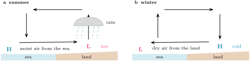
The monsoon of South and South-East Asia starts in late May or early June, progresses north-eastward and ends in late September or early October. Before it, the lands around the Arabian Sea heat up: in June the surface sends about $160\,\mathrm{W}/\mathrm{m}^{2}$ of heat into the air over the arid north-west of India, Pakistan and the Middle East, and a shallow heat low forms there, reaching only to about $1.5\,\mathrm{km}$, with little rain; a weak heat low, as in the drought year 1987, means a weak pull on the moist air of the ocean. From it an elongated trough of low pressure, the monsoon trough, runs to the head of the Bay of Bengal; its north–south oscillations bring the active spells and the breaks of the season. Over India as a whole the rain of June to September averages $88\,\mathrm{cm}$, with a standard deviation of $9\,\mathrm{cm}$, about $10\,\%$: a season within $10\,\%$ of the long-period average is called normal. On the Kerala coast, where the national weather service declares the onset of the monsoon from the rainfall of fourteen stations, the winds and the satellite-measured outgoing infrared radiation, the average rainfall is $556\,\mathrm{mm}$ in June and $659\,\mathrm{mm}$ in July.

The West African monsoon brings moist south-westerly winds from the Gulf of Guinea, progressing northward from May to September; its rain peaks near $12{}^{\circ}$ N in late August and September and retreats from October.

A monsoon is regular in its timing, irregular in its amount, and the year-to-year swings of the tropical Pacific are among the causes. El Niño years tend to leave India short of rain: the droughts of 1904, 1972 and 1987 came with El Niño. The link is not certain: in 1997 a strong El Niño coincided with a positive phase of the Indian Ocean Dipole, a mode met below, and India had a near-normal monsoon.

23.3 El Niño and the Southern Oscillation

The Year 1 volume described the Walker circulation: air rising over the warm western Pacific, flowing east aloft, sinking over the cool eastern Pacific and returning west with the trade winds. In the ocean below, the trade winds pile warm water in the west, where the thermocline is deep, and draw cold water up along the equator in the east, where it is shallow. This state is not fixed.

Definition 23.5 (El Niño–Southern Oscillation; El Niño; La Niña; Southern Oscillation)

The El Niño–Southern Oscillation (ENSO) is the coupled ocean–atmosphere mode of the tropical Pacific: coherent year-to-year variations of the sea-surface temperature, the convective rainfall, the surface pressure and the circulation along the equatorial Pacific, with preferred time scales of two to about seven years. El Niño is its warm phase, a warming of the sea surface of the central and east-central equatorial Pacific; La Niña is its cold phase, a cooling of the same region. The Southern Oscillation is its atmospheric part, a see-saw of surface pressure between the western and the eastern tropical Pacific: during El Niño the pressure is higher than average over Indonesia and the western Pacific and lower over the eastern Pacific, and the reverse during La Niña.

During El Niño, the easterly trade winds weaken along the equator, and in the west the low-level winds may even blow from the west; the warm water of the west spreads east, and the deep convection and its rain follow it, leaving Indonesia and northern Australia drier. The sea surface of the east-central Pacific is typically $1.5\text{ to }2.5\,{}^{\circ}\mathrm{C}$ warmer than average, and the thermocline there lies at $150\text{ to }175\,\mathrm{m}$, deeper than usual. During La Niña the trade winds strengthen across the whole basin, the sea surface is $1\text{ to }2\,{}^{\circ}\mathrm{C}$ colder than average, and the thermocline in the east rises to $50\text{ to }100\,\mathrm{m}$. The Walker circulation weakens during El Niño and strengthens during La Niña. Episodes typically recur every three to five years, at intervals that have ranged from two to seven; an El Niño typically lasts nine to twelve months, a La Niña one to three years. Both tend to develop between March and June, to peak between December and April and to weaken between May and July; their effects are strongest from December to April, when the equatorial sea surface is warmest.

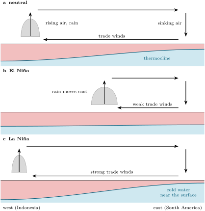
The names come from different centuries and different sciences. Fishermen of the coast of South America noticed a warming of their coastal waters around Christmas that disrupted the fishery, and called it El Niño, the boy child. Sir Gilbert Walker discovered the Southern Oscillation in the atmosphere, without linking it to the ocean. Only in the late 1960s did Jacob Bjerknes and others see that the two were one phenomenon. The terms La Niña and neutral gained prominence in the 1980s.

History — The boy child of the fishermen

Off the dry coast of Peru, the cold water that the winds draw up along the shore is rich in nutrients and feeds a productive fishery. Its fishermen knew a warming that came around Christmas, when the fish became scarce, and gave it the name of the child of the season. The anchovy catch of Peru still follows ENSO: in a recent analysis, prolonged high temperature anomalies made an extremely low catch more than nine times likelier, with a median fall of the catch of about $60\,\%$; the strong El Niño of 1997–98 stands out in the record.

Why does the system swing at all? Because the ocean and the atmosphere of the equatorial Pacific reinforce each other’s anomalies.

Definition 23.6 (Bjerknes feedback)

The Bjerknes feedback is the positive feedback between the sea-surface temperature, the winds and the ocean currents of the equatorial Pacific: a warming of the east weakens the east–west contrast of temperature and pressure, hence the trade winds; weaker trade winds let the warm water of the west spread east and bring up less cold water in the east, which warms the east further. The same loop amplifies a cooling.

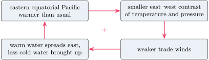
A positive feedback explains how an anomaly grows, not how it starts or ends. In one current account, an El Niño begins when random fluctuations of the trade winds weaken the equatorial currents that keep the warm water in the west; the warm pool spreads east, the convection follows it, the Bjerknes feedback takes over and the event grows. La Niña events, in the same account, are triggered by a preceding El Niño. The simplest models that make the system oscillate, the recharge oscillator among them, couple two quantities: the sea-surface temperature anomaly of the central Pacific and the volume of warm upper-ocean water stored along the equator. The temperature anomaly drains or refills that store through the winds it drives, and the store, through the depth of the thermocline, prepares the next phase. Exercise 23.10 solves such a pair of equations.

To follow ENSO, the monitoring centres use indices.

Definition 23.7 (Niño-3.4 index; Oceanic Niño Index)

The Niño-3.4 index is the monthly anomaly of the sea-surface temperature averaged over the region $5{}^{\circ}$ N–$5{}^{\circ}$ S, $170{}^{\circ}$ W–$120{}^{\circ}$ W, relative to the climatology of a 30-year base period centred on the year, updated every five years. The Oceanic Niño Index (ONI) is its three-month running mean. An El Niño (a La Niña) episode is a run of at least five consecutive overlapping three-month seasons with the ONI at or above $+0.5\,{}^{\circ}\mathrm{C}$ (at or below $-0.5\,{}^{\circ}\mathrm{C}$).

The seasons overlap: DJF, JFM, FMA and so on, each the mean of three months, each sharing two months with the next. A second index, the Southern Oscillation Index, follows the atmosphere: it is computed from the departures of the pressure difference between Tahiti and Darwin, negative during El Niño, positive during La Niña. Since February 2026 the official index for monitoring ENSO is a relative ONI, computed from the Niño-3.4 anomaly minus the mean anomaly of the whole tropical ocean between $20{}^{\circ}$ N and $20{}^{\circ}$ S, then rescaled to the amplitude of the ONI. Being measured against the whole tropics, it depends less on the choice of base period while the oceans warm, and it is better related to the rainfall of the tropical Pacific. In September 2026 the relative anomaly of the Niño-3.4 region was $2.08\,{}^{\circ}\mathrm{C}$, against the $2.56\,{}^{\circ}\mathrm{C}$ of Example 23.3: about half a degree of the traditional anomaly was the warmth of the tropical oceans as a whole.

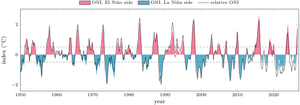
Counted with the five-season rule on the table of the Climate Prediction Center, the ONI shows 25 El Niño and 21 La Niña episodes between 1950 and the summer of 2026. The strongest El Niño peaks were $2.4\,{}^{\circ}\mathrm{C}$ in late 1997 and $2.6\,{}^{\circ}\mathrm{C}$ in late 2015. The two indices diverge most in recent years: in July–September 2026 the ONI stood at $2.2\,{}^{\circ}\mathrm{C}$ and the relative index at $1.7\,{}^{\circ}\mathrm{C}$.

Figures as of 2026

In its discussion of 8 October 2026 the Climate Prediction Center kept its El Niño advisory: the relative Niño-3.4 anomaly had reached $+2.1\,{}^{\circ}\mathrm{C}$ in September, parts of the eastern equatorial Pacific were more than $4\,{}^{\circ}\mathrm{C}$ above average, the water at depth in the east more than $10\,{}^{\circ}\mathrm{C}$ above, and the Southern Oscillation indices were significantly negative. A strong-to-very strong El Niño was judged likely through January–March 2027, and the chance that the relative index would exceed $2.5\,{}^{\circ}\mathrm{C}$, beyond every event since 1950, was put at $83\,\%$ for October–December.

23.4 The North Atlantic Oscillation and teleconnections

Definition 23.8 (North Atlantic Oscillation)

The North Atlantic Oscillation (NAO) is the leading mode of atmospheric variability over the North Atlantic: a see-saw of sea-level pressure between the Icelandic Low and the Azores High. Its index is positive when both are stronger than average, so that the pressure difference between them is large, and negative when both are weaker.

The NAO steers the westerlies of the previous chapter. In its positive phase the larger pressure difference drives a stronger Atlantic jet stream and shifts the storm track north: northern Europe has a stormier, wetter and milder winter, southern Europe a drier one, eastern North America fewer outbreaks of cold air, and Greenland a colder winter. The negative phase reverses these anomalies. In the late eighteenth century a missionary already noted that mild winters in Greenland came with severe ones in Denmark, and the reverse.

The NAO is one of the most prominent patterns of the atmosphere in every season, and it is strongly correlated with another mode, the Arctic Oscillation. It also varies over decades: the negative phase dominated from the mid-1950s to the winter of 1978–79, and the positive phase from 1979–80 to 1994–95.

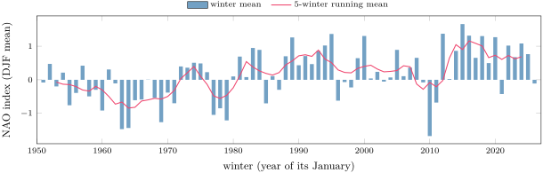
The NAO, ENSO and the other modes act far from where they are measured.

Definition 23.9 (Teleconnection)

A teleconnection is an association between climate variables at widely separated, fixed places, linked by physical processes along paths in the atmosphere or the ocean, such as trains of Rossby waves, shifts of the jet stream and the storm tracks, or changes of the Walker circulation.

During El Niño the rainfall of the tropics changes from Indonesia to South America, about half way round the world, and from the tropics the anomalies travel to the middle latitudes by the paths of the definition; the Indian monsoon of the previous section is one of their ends. Other modes have been named in each ocean: the Indian Ocean Dipole, an east–west see-saw of sea-surface temperature in the tropical Indian Ocean whose positive phase cools the sea off Sumatra and Java and warms it off Somalia, which develops in the northern summer, matures in autumn, and changes the rain of Australia, South-East Asia and East Africa; the Southern Annular Mode, the changes of strength and latitude of the westerly belt around Antarctica; and the decadal variability of the Pacific, slower than ENSO.

23.5 The ocean as memory

Chapter 22 found that the atmosphere forgets its weather within about two weeks. A climate anomaly that lasts a season must be stored somewhere, and the obvious store is the mixed layer of the ocean: a deeper mixed layer holds more heat and has more thermal inertia. The simplest model treats the anomaly as a reservoir that leaks heat to the atmosphere.

Proposition 23.10 (Damping time of a mixed-layer anomaly)

Let a mixed layer of depth $h$, density $\rho$ and specific heat $c_p$ carry a temperature anomaly $T'$, and let the surface lose an extra heat flux $\alpha T'$ per unit area to the atmosphere, with $\alpha > 0$. Then, without other forcing,

$$T'(t) = T'(0)\,\mathrm{e}^{-t/\tau}, \qquad \tau = \frac{\rho\,c_p\,h}{\alpha} .$$

Example 23.11 (The memory of a mid-latitude ocean)

Over the oceans of the middle latitudes, the surface heat flux responds to a sea-surface temperature anomaly with a mean $\alpha = 16.1\,\mathrm{W}\,\mathrm{m}^{-2}\,\mathrm{K}^{-1}$. For a mixed layer $50\,\mathrm{m}$ deep, with $\rho = 1025\,\mathrm{kg}/\mathrm{m}^{3}$ and $c_p = 3992\,\mathrm{J}\,\mathrm{kg}^{-1}\,\mathrm{K}^{-1}$, $\tau = 1025 \times 3992 \times 50/16.1 = 1.27 \times 10^{7}\,\mathrm{s} = 147\,\mathrm{d}$, nearly five months; a layer $100\,\mathrm{m}$ deep remembers twice as long.

Real anomalies are also forced, every day, by the weather: random fluxes of heat that, alone, would make a white noise, with no memory from one month to the next. Added to the damping, they give the equation $\mathrm{d}T'/\mathrm{d}t = -T'/\tau + F(t)$ with a random $F$: the ocean sums the random forcing over a time of the order of $\tau$ and forgets it beyond. The result is called a red noise. Its lag correlation, the correlation between the anomaly and itself some time later, falls as $\mathrm{e}^{-\text{lag}/\tau}$ (admitted), and slow variations are much stronger in it than in the forcing. This stochastic model of the memory of the ocean is the standard reference against which the persistence of real anomalies is measured, a source of predictability beyond the time scales of weather; since the depth of the mixed layer sets the memory, the shoaling of mixed layers projected for this century implies a shorter one.

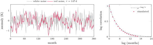
ENSO needs more than this passive memory. Its anomalies involve not only the mixed layer but the whole warm layer above the thermocline, which moves by tens of metres, and the winds that the anomalies drive feed back on the ocean through the Bjerknes loop. The ocean supplies the slowness, the atmosphere the coupling; neither alone makes the oscillation. The slowness is what the forecasters of October 2026 relied on when they judged a strong El Niño likely to last through January–March 2027.

Exercises

Data for the exercises, unless stated otherwise: seawater $\rho = 1025\,\mathrm{kg}/\mathrm{m}^{3}$ and $c_p = 3992\,\mathrm{J}\,\mathrm{kg}^{-1}\,\mathrm{K}^{-1}$; air $c_p = 1004.5\,\mathrm{J}\,\mathrm{kg}^{-1}\,\mathrm{K}^{-1}$; $g = 9.81\,\mathrm{m}\,\mathrm{s}^{-2}$; the damping coefficient of the surface heat flux $\alpha = 16.1\,\mathrm{W}\,\mathrm{m}^{-2}\,\mathrm{K}^{-1}$; a month is $365.25/12 = 30.44$ days.

Exercise 23.1 ★

In the Niño-3.4 region the mean sea-surface temperature was $29.27\,{}^{\circ}\mathrm{C}$ in September 2026 and $28.79\,{}^{\circ}\mathrm{C}$ in September 1997; the climatologies used for those two Septembers were $26.71\,{}^{\circ}\mathrm{C}$ and $26.73\,{}^{\circ}\mathrm{C}$. (a) Compute the two anomalies. (b) Which September was warmer, and which anomaly larger? (c) Why is the climatology not the same for the two years?

Solution

Solution of Exercise 23.1.

(a) $29.27 - 26.71 = 2.56\,{}^{\circ}\mathrm{C}$ in 2026; $28.79 - 26.73 = 2.06\,{}^{\circ}\mathrm{C}$ in 1997. (b) September 2026 was both the warmer month, by $0.48\,{}^{\circ}\mathrm{C}$, and the larger anomaly, by $0.50\,{}^{\circ}\mathrm{C}$. (c) Each year is compared with a 30-year base period centred on it, moved every five years; the September climatology of the 1980s and 1990s differs slightly from that of the 2010s and 2020s.

Exercise 23.2 ★

The monthly Niño-3.4 anomalies of June to December 2023 were 0.79, 0.95, 1.28, 1.55, 1.68, 2.01 and $2.02\,{}^{\circ}\mathrm{C}$. (a) Compute the ONI of the seasons JJA to OND. (b) The table of the Climate Prediction Center gives 1.0, 1.3, 1.5, 1.7 and 1.9. Compare. (c) In which season did the ONI first reach the threshold of a strong event, $1.5\,{}^{\circ}\mathrm{C}$?

Solution

Solution of Exercise 23.2.

(a) JJA: $(0.79 + 0.95 + 1.28)/3 = 1.007$; JAS: $(0.95 + 1.28 + 1.55)/3 = 1.260$; ASO: $(1.28 + 1.55 + 1.68)/3 = 1.503$; SON: $(1.55 + 1.68 + 2.01)/3 = 1.747$; OND: $(1.68 + 2.01 + 2.02)/3 = 1.903$, all in ${}^{\circ}\mathrm{C}$. (b) Rounded to one decimal: 1.0, 1.3, 1.5, 1.7, 1.9, the values of the table. (c) In ASO 2023, at 1.5.

Exercise 23.3 ★

In a given month the surface pressure is above average at Darwin and below average at Tahiti. (a) What is the sign of the Southern Oscillation Index? (b) Which phase of ENSO does it suggest? (c) What do you expect for the trade winds over the eastern equatorial Pacific, and for the rainfall over Indonesia?

Solution

Solution of Exercise 23.3.

(a) The index follows the departure of the pressure at Tahiti minus that at Darwin: below average at Tahiti and above at Darwin, it is negative. (b) El Niño. (c) Weaker easterly trade winds, even westerly winds near the surface in the west, and less rain than usual over Indonesia, since the deep convection has moved east.

Exercise 23.4 ★

(a) The rainfall of June to September 2018 over India was $804.1\,\mathrm{mm}$, against a long-period average of $880.6\,\mathrm{mm}$. Compute it as a percentage of the average and classify the season. (b) On the Kerala coast the averages for June, July, August and September are 556, 659, 427 and $252\,\mathrm{mm}$. What fraction of the season’s rain falls in July?

Solution

Solution of Exercise 23.4.

(a) $804.1/880.6 = 91.3\,\%$ of the average: within 90 to $110\,\%$, a normal season, though in its lower part. (b) The season totals $556 + 659 + 427 + 252 = 1894\,\mathrm{mm}$; July brings $659/1894 = 34.8\,\%$ of it, more than a third.

Exercise 23.5 ★★

(a) Compute the damping time of an anomaly in mixed layers $50\,\mathrm{m}$ and $100\,\mathrm{m}$ deep. (b) Compute, for each, the lag correlation of the anomaly after one month. (c) Climate models project shallower mixed layers in a warmer climate. What does that do to the memory of the ocean?

Solution

Solution of Exercise 23.5.

(a) $\tau = 1025 \times 3992 \times 50/16.1 = 1.271 \times 10^{7}\,\mathrm{s} = 147.1\,\mathrm{d}$ for $50\,\mathrm{m}$, and twice that, $294.2\,\mathrm{d}$, for $100\,\mathrm{m}$. (b) $\mathrm{e}^{-30.44/147.1} = 0.813$ and $\mathrm{e}^{-30.44/294.2} = 0.902$. (c) The damping time is proportional to $h$: a shallower mixed layer stores less heat for the same flux and forgets an anomaly faster, so the ocean’s memory, and the predictability it gives, decline.

Exercise 23.6 ★★

A sea-surface temperature anomaly of $+1.2\,\mathrm{K}$ is observed over a mixed layer $50\,\mathrm{m}$ deep. (a) Without further forcing, what anomaly remains after three months, and after six? (b) Such a forecast, which only lets the present anomaly decay, is called a persistence forecast. Why is it better than assuming no anomaly at all, and why does it get worse with time?

Solution

Solution of Exercise 23.6.

(a) Three months are 91.3 days: $1.2 \times \mathrm{e}^{-91.3/147.1} = 0.65\,\mathrm{K}$; six months are 182.6 days: $1.2 \times \mathrm{e}^{-182.6/147.1} = 0.35\,\mathrm{K}$. (b) The anomaly decays slowly, so it is a better guess of next month’s anomaly than zero. But the random forcing adds new anomalies every day, unknown at the time of the forecast; as the initial anomaly decays, they take an ever larger share, and the forecast drifts towards the climatology, where it no longer helps.

Exercise 23.7 ★★

In June the ground of the deserts of north-west India and Pakistan sends about $160\,\mathrm{W}/\mathrm{m}^{2}$ of heat into the air. (a) How much energy is that per square metre and per day? (b) If it all stayed in the layer between the ground at $1000\,\mathrm{hPa}$ and $850\,\mathrm{hPa}$, how fast would that layer warm? (c) The heat low does not in fact warm at that rate week after week. Name two ways the heat can leave the layer.

Solution

Solution of Exercise 23.7.

(a) $160 \times 86\,400 = 1.38 \times 10^{7}\,\mathrm{J}$, $13.8\,\mathrm{MJ}$ per square metre and per day. (b) The layer holds $(1000 - 850) \times 100/9.81 = 1529\,\mathrm{kg}$ of air per square metre, with a heat capacity of $1529 \times 1004.5 = 1.536 \times 10^{6}\,\mathrm{J}\,\mathrm{m}^{-2}\,\mathrm{K}^{-1}$; it would warm by $1.38 \times 10^7/1.536 \times 10^6 = 9.0\,\mathrm{K}$ a day. (c) The layer radiates heat in the infrared, to space and to the air above; and the warm air rises and mixes with the layer above it, or is carried away by the winds, among them the inflow of cooler air the heat low itself draws in.

Exercise 23.8 ★★

The monthly NAO index was $-1.93$ in December 2009, $-1.11$ in January 2010 and $-1.98$ in February 2010. (a) Compute the winter mean. (b) Over 1951–2026 the winter means range from $-1.67$ to $+1.66$. Place this winter. (c) What winter weather would you expect in northern Europe, in southern Europe and in the eastern United States?

Solution

Solution of Exercise 23.8.

(a) $(-1.93 - 1.11 - 1.98)/3 = -1.673$, about $-1.67$. (b) It is the lowest winter of the record. (c) A strongly negative NAO: a weak Icelandic Low and Azores High, a weaker jet and a storm track further south than usual; a cold, dry winter in northern Europe, a wet one in southern Europe, and more outbreaks of cold air in the eastern United States.

Exercise 23.9 ★★

A region belongs to the global monsoon domain when the mean rain of its local summer exceeds that of its winter by more than $2.5\,\mathrm{mm}$ a day. (a) An invented station of the Northern Hemisphere receives $9.3\,\mathrm{mm}$ a day on average in June–August and $0.4\,\mathrm{mm}$ a day in December–February. Is it in the domain? (b) An invented station of the Southern Hemisphere receives $4.2\,\mathrm{mm}$ a day in June–August and $6.1\,\mathrm{mm}$ a day in December–February. Is it? (c) On the Kerala coast the mean rain of June to September (122 days) is 556, 659, 427 and $252\,\mathrm{mm}$ month by month. Compute its mean daily rate, and the winter rate above which Kerala, taking June–September as its summer, would fall outside the domain. (d) Why does the criterion use the difference between the seasons and not the total rain of the year?

Solution

Solution of Exercise 23.9.

(a) $9.3 - 0.4 = 8.9\,\mathrm{mm}$ a day, more than 2.5: in the domain. (b) In the Southern Hemisphere the summer is December–February: $6.1 - 4.2 = 1.9\,\mathrm{mm}$ a day, less than 2.5: outside it, although it rains more there than at most places of the domain. (c) $1894/122 = 15.5\,\mathrm{mm}$ a day; Kerala would be outside only if its winter rate exceeded $15.5 - 2.5 = 13.0\,\mathrm{mm}$ a day. (d) A monsoon is a seasonal reversal: a wet place that is wet all year round, like the second station, has no monsoon, and a dry place with a short, intense rainy season has one.

Exercise 23.10 ★★★

A simple recharge oscillator writes the Niño-3.4 temperature anomaly $T$ and the anomaly $H$ of the warm water stored along the equator as $\dot T = aH$, $\dot H = -bT$, with $a, b > 0$. (a) Show that $T$ oscillates, with the period $2\pi/\sqrt{ab}$. (b) What product $ab$ gives a period of four years? (c) With damping, $\dot T = aH - rT$ and $\dot H = -bT - rH$, show that $(T\,\mathrm{e}^{rt}, H\,\mathrm{e}^{rt})$ obeys the undamped equations. With $r = 0.25$ per year, by what factor does the amplitude fall in one period? (d) What must keep the real oscillation going?

Solution

Solution of Exercise 23.10.

(a) Differentiating, $\ddot T = a\dot H = -abT$: the equation of a harmonic oscillator of angular frequency $\omega = \sqrt{ab}$, and period $2\pi/\sqrt{ab}$. (b) $2\pi/\sqrt{ab} = 4$ gives $ab = (2\pi/4)^2 = 2.47\,\mathrm{yr}^{-2}$. (c) With $T = u\,\mathrm{e}^{-rt}$, $H = v\,\mathrm{e}^{-rt}$, $\dot T = (\dot u - ru)\,\mathrm{e}^{-rt} = (av - ru)\,\mathrm{e}^{-rt}$, so $\dot u = av$, and likewise $\dot v = -bu$: $(u, v)$ oscillates without damping, and $(T, H)$ is that oscillation multiplied by $\mathrm{e}^{-rt}$. In one period the amplitude falls by $\mathrm{e}^{-0.25 \times 4} = \mathrm{e}^{-1} = 0.37$. (d) A forcing: the random fluctuations of the trade winds, which kick the system again and again, and the Bjerknes feedback, which makes the damping weaker or even negative.

Exercise 23.11 ★★★

The Niño-3.4 region extends $10{}^{\circ}$ in latitude and $50{}^{\circ}$ in longitude along the equator (take an Earth radius of $6371\,\mathrm{km}$). (a) Compute its area. (b) How much heat does it take to warm a layer $100\,\mathrm{m}$ deep over that area by $2\,\mathrm{K}$? (c) What extra surface heat flux, sustained over six months, would supply it? (d) During El Niño the trade winds weaken and the thermocline in the east deepens. Where else can the heat come from?

Solution

Solution of Exercise 23.11.

(a) $A = R^2 \,\Delta\lambda\,(\sin5{}^{\circ} - \sin(-5{}^{\circ})) = (6.371 \times 10^6)^2 \times 0.8727 \times 0.1743 = 6.17 \times 10^{12}\,\mathrm{m}^{2}$. (b) $Q = 1025 \times 3992 \times 100 \times 2 \times 6.17 \times 10^{12} = 5.05 \times 10^{21}\,\mathrm{J}$. (c) Six months are $182.6 \times 86\,400 = 1.578 \times 10^{7}\,\mathrm{s}$; per square metre, $8.18 \times 10^8/1.578 \times 10^7 = 51.9\,\mathrm{W}/\mathrm{m}^{2}$, sustained for half a year. (d) From the ocean itself: weaker trades bring up less cold water in the east, and the warm water of the west, stored above the deeper thermocline, spreads east; much of the warming can come from heat already in the ocean, moved rather than gained.

Exercise 23.12 ★★★

Treat the Bjerknes feedback as a loop that returns, as extra warming, a fraction $g$ of any warming that passes through it. (a) A burst of westerly wind warms the east by $0.3\,\mathrm{K}$. Show that the total warming is $0.3/(1 - g)$, and compute it for $g = 0.5$, 0.8 and 0.9. (b) What happens if $g \geq 1$, and what must then limit the event? (c) Why should $g$ be largest in the season when the equatorial Pacific is warmest?

Solution

Solution of Exercise 23.12.

(a) The loop returns $0.3g$, then $0.3g^2$, and so on: the total is $0.3(1 + g + g^2 + \dots) = 0.3/(1 - g)$, a geometric series that converges for $g < 1$: $0.6\,\mathrm{K}$, $1.5\,\mathrm{K}$ and $3.0\,\mathrm{K}$ for $g = 0.5$, 0.8 and 0.9. (b) The series diverges: the anomaly would grow without limit; the growth must be stopped by processes the loop leaves out, the damping by the surface heat flux and the draining of the warm-water store that the recharge oscillator describes. (c) The warmer the sea surface, the more readily a small warming triggers deep convection and rain, whose heating drives the winds; that is the season in which the effects of ENSO are strongest.

Problem 23.1

Weekend problem — Counting El Niños

From monthly sea temperatures to the record of El Niño since 1950, and to the ocean that makes it possible. Use the data of the exercises.

Part I — From months to seasons. The monthly Niño-3.4 anomalies from April 1997 to January 1998 were 0.26, 0.75, 1.13, 1.52, 1.80, 2.06, 2.26, 2.42, 2.36 and $2.33\,{}^{\circ}\mathrm{C}$.

1. Compute the ONI of the season AMJ 1997.
2. Compute the ONI of MJJ, JJA and JAS.
3. Compute the ONI of ASO, SON, OND and NDJ.
4. The table of the Climate Prediction Center gives 0.7, 1.1, 1.5, 1.8, 2.0, 2.2, 2.3 and 2.4 for these eight seasons. Compare.
5. Why does the index average three months instead of using single months?
6. In which season did the 1997 event become strong ($\geq 1.5\,{}^{\circ}\mathrm{C}$), and at what value did it peak?

Part II — The five-season rule. The ONI of the Climate Prediction Center for 2018 to 2020 reads, season by season from DJF to NDJ: 2018: $-0.7$, $-0.7$, $-0.5$, $-0.3$, $-0.1$, 0.1, 0.2, 0.3, 0.5, 0.8, 1.0, 1.1; 2019: 1.0, 0.9, 0.9, 0.8, 0.7, 0.6, 0.4, 0.2, 0.3, 0.5, 0.7, 0.8; 2020: 0.7, 0.7, 0.6, 0.3, 0.0, $-0.2$, $-0.3$, $-0.4$, $-0.8$, $-1.0$, $-1.1$, $-1.1$; then DJF 2021 $-1.0$ and JFM 2021 $-0.9$. The relative ONI reads, from SON 2018: 0.62, 0.82, 0.78; 2019: 0.68, 0.64, 0.57, 0.53, 0.37, 0.24, 0.04, $-0.12$, $-0.01$, 0.15, 0.29, 0.22; 2020: 0.14, 0.10, 0.02, $-0.25$, $-0.55$, $-0.72$, $-0.76$, $-0.85$, $-1.16$, $-1.37$, $-1.46$, $-1.39$.

7. Find the El Niño episodes of 2018–2020 under the ONI: first and last season of each.
8. How many seasons does each last?
9. In which season does the next La Niña begin under the ONI, and why do you need the values of 2021 to be sure of it?
10. Find the El Niño episodes under the relative ONI, and the first season of the La Niña.
11. Is the event of late 2019 an El Niño under the relative ONI? Explain the difference between the two indices in 2019.

Part III — Strong El Niños. The El Niño episodes since 1950 whose peak ONI reached at least $1.5\,{}^{\circ}\mathrm{C}$ began in the seasons MAM 1957, AMJ 1965, AMJ 1972, AMJ 1982, JAS 1986, AMJ 1991, AMJ 1997, JJA 2009, SON 2014, AMJ 2023 and MAM 2026, with peaks of 1.7, 1.8, 1.8, 2.1, 1.5, 1.5, 2.4, 1.5, 2.6, 2.0 and, at JAS 2026, $2.2\,{}^{\circ}\mathrm{C}$ and rising. Count in years, from the year in which each began.

12. How many strong episodes are there?
13. List the intervals between the starts of successive strong episodes.
14. Which interval is the shortest, which the longest?
15. Compute the mean interval in two ways: as the mean of the intervals, and as the time from the first start to the last divided by the number of intervals. Why do they agree?
16. The 2026 event was still growing when the data stop. Why does it nevertheless count as a strong episode, and why can no later data change its start?
17. The FAQ of the Climate Prediction Center says El Niño and La Niña occur every 3 to 5 years. Is the mean interval of the strong ones consistent with that?

Part IV — Why ENSO needs the ocean. Take a mixed layer $50\,\mathrm{m}$ deep and an air column of $1000\,\mathrm{hPa}$.

18. Compute the damping time of a mixed-layer anomaly.
19. Compute the heat capacity per square metre of the mixed layer and of the whole air column above it.
20. What depth of seawater has the heat capacity of the whole atmosphere above it?
21. Compute the damping time of an anomaly carried by the air column alone, with the same $\alpha$.
22. Why can the ocean carry an ENSO anomaly from one season to the next, and the atmosphere not?
23. To sum up: how many years, on average, separate the starts of successive strong El Niño episodes since 1950?

Solution

Solution of Problem 23.1.

1. $(0.26 + 0.75 + 1.13)/3 = 0.713\,{}^{\circ}\mathrm{C}$. 2. MJJ $(0.75 + 1.13 + 1.52)/3 = 1.133$; JJA $(1.13 + 1.52 + 1.80)/3 = 1.483$; JAS $(1.52 + 1.80 + 2.06)/3 = 1.793$. 3. ASO $(1.80 + 2.06 + 2.26)/3 = 2.040$; SON $(2.06 + 2.26 + 2.42)/3 = 2.247$; OND $(2.26 + 2.42 + 2.36)/3 = 2.347$; NDJ $(2.42 + 2.36 + 2.33)/3 = 2.370$. 4. Rounded to one decimal, 0.7, 1.1, 1.5, 1.8, 2.0, 2.2, 2.3 and 2.4: the table. 5. A single month carries weather noise; ENSO lasts many months, and the mean of three removes much of the noise while keeping the slow signal. 6. In JJA 1997, at 1.483, rounded to 1.5; it peaked at 2.4 in NDJ. 7. From ASO 2018 to MJJ 2019, and from SON 2019 to FMA 2020. 8. Ten seasons, and six. 9. In ASO 2020; within 2020 only four seasons, ASO to NDJ, are at or below $-0.5$, one short of the rule, and DJF 2021 completes it. 10. One El Niño, SON 2018 to MAM 2019, seven seasons (AMJ 2019 falls to 0.37); the La Niña starts in AMJ 2020 ($-0.55$), four seasons before the ONI places it, in ASO. 11. No: the relative index never exceeds 0.29 in late 2019. The whole tropical ocean was then warmer than its base period by about half a degree; the Niño-3.4 region was warm in absolute terms, but hardly warmer than the tropics around it. 12. Eleven. 13. 8, 7, 10, 4, 5, 6, 12, 5, 9 and 3 years. 14. The shortest is 3 years (2023 to 2026), the longest 12 (1997 to 2009). 15. $69/10 = 6.9$ years either way: the sum of successive intervals is the time from the first start to the last, $2026 - 1957 = 69$ years. 16. It has already lasted five seasons, MAM to JAS, at or above $0.5\,{}^{\circ}\mathrm{C}$, and peaked at 2.2, above 1.5; its start, MAM 2026, is the first season of the run, and later seasons can only extend the run, not move its beginning. 17. No, and it need not be: the 25 episodes of all strengths come about every three years, as the FAQ says; the strong ones are a subset, so they are rarer, and their intervals range from 3 to 12 years. 18. $\tau = 1025 \times 3992 \times 50/16.1 = 1.27 \times 10^{7}\,\mathrm{s} = 147\,\mathrm{d}$. 19. Mixed layer: $1025 \times 3992 \times 50 = 2.05 \times 10^{8}\,\mathrm{J}\,\mathrm{m}^{-2}\,\mathrm{K}^{-1}$; air column: $(10^5/9.81) \times 1004.5 = 10\,194 \times 1004.5 = 1.02 \times 10^{7}\,\mathrm{J}\,\mathrm{m}^{-2}\,\mathrm{K}^{-1}$, 20 times less. 20. $1.024 \times 10^7/(1025 \times 3992) = 2.5\,\mathrm{m}$ of seawater. 21. $1.024 \times 10^7/16.1 = 6.36 \times 10^{5}\,\mathrm{s} = 7.4$ days. 22. An anomaly of the air alone is damped in about a week, one of the mixed layer in about five months, and the warm layer above the thermocline is deeper still: only the ocean holds heat long enough to carry an anomaly from one season to the next, while the atmosphere supplies the winds that couple the two. 23. Since 1950, strong El Niño episodes have begun on average every 6.9 years, about seven.