24Climate Archives and Proxies

In a paper of 1955 a young geochemist reported the oxygen isotopes of the tiny shells of foraminifera picked from cores of the ocean floor, and found in them fifteen glacial–interglacial cycles over the last $600\,000$ years. He read them mostly as temperature: he attributed only about a fifth of the swings to the ice stored on land. Eighteen years later, Shackleton and Opdyke concluded the opposite: the main effect was the storage of isotopically light water in the ice sheets. The same shells, the same numbers, two readings. A shell of calcite records the temperature of the water it grew in and the composition of that water, and the composition of sea water depends on how much ice there is on land. This chapter is about such records, the archives that keep them, the proxies read from them, how they are calibrated against thermometers and how they are dated, and about the art of telling apart two signals carried by one shell.

You already know

From the school volumes: climate archive and proxy, ice core, glacial period and interglacial, the Last Glacial Maximum (about $23\,000$ to $19\,000$ years ago), pollen analysis. From the Year 1 volume: radiometric dating, the radiocarbon age and its calibration curve; calcareous ooze, made of coccoliths and the shells of foraminifera. From Chapter 4: the isotope reference standards VSMOW and VPDB (Definition 4.11) and the meteoric water line, $\delta\mathrm{D} \approx 8\,\delta^{18}\mathrm{O} + 10$ (Proposition 4.12). From the chemistry books: the $\delta$ value and the fractionation factor. From the mathematics books: the least-squares line.

24.1 Archives and proxies

Instruments have measured the climate only recently. Everything earlier is read from materials that grew or settled layer by layer while the climate acted on them: snow turning to ice on the polar ice sheets, shells raining onto the ocean floor, the rings of trees, corals, the deposits of caves, the mud of lakes. The school volumes called them archives and the quantities measured in them proxies; we now need sharper words.

Definition 24.1 (Climate archive; climate proxy)

A climate archive is a natural material that accumulates progressively, layer upon layer or ring upon ring, and preserves physical, chemical or biological characteristics of the environment in which each part formed. A climate proxy is a quantity measured in an archive that depends on a climate variable, such as a temperature, an amount of rain or a volume of ice, through a relation that can be calibrated, and so stands in for a measurement of that variable that was never made.

Three properties decide what an archive can tell: its resolution (the time span covered by one sample), its reach (how far back it goes) and how it is dated. An archive with annual layers can be read year by year and dated by counting; the others need radiometric ages or comparison with a dated record. The table below compares the archives of this chapter.

A proxy is never a pure measure of one variable. The width of a tree ring depends on the warmth of the summer and on the rain; the $\delta^{18}$O of a shell on the temperature of the water and on its isotopic composition. The work of the palaeoclimatologist is to find a proxy whose dependence on the variable sought is strong and known, to measure the other influences independently, and to date the sample.

24.2 Oxygen isotopes in carbonate shells

Foraminifera are single-celled protists, many of which build a shell of calcite; the planktonic species float in the surface waters, the benthic ones live on or in the sediment of the sea floor. Their shells accumulate in the calcareous oozes of the Year 1 volume, and the $\delta^{18}$O of the calcite can be measured on a few shells picked from each centimetre of a core.

History — Two readings of one record

Urey calculated in 1947 how the fractionation of oxygen between calcite and water depends on temperature, and proposed that carbonates could record the temperature at which they formed. Cesare Emiliani, then his student, measured $\delta^{18}$O in foraminifera from piston cores of the world’s oceans and published in 1955 a record with 15 glacial–interglacial cycles over $600\,000$ years, attributing about $20\,\%$ of the variation to the volume of ice. In 1973 Shackleton and Opdyke concluded that the storage of isotopically light water in the ice sheets was the main effect. The vital effects, the departures of a species from equilibrium, and the exchange of oxygen with pore water after burial are usually not very important for the shells of the last few million years; the isotopic composition of the water is.

Temperature

Calcite that grows in equilibrium with water is richer in ¹⁸O than the water, and the colder the water, the larger the enrichment, as Urey’s calculation showed. Several empirical calibrations relate temperature to the difference between the $\delta^{18}$O of the calcite, on the VPDB scale, and that of the water, on the VSMOW scale. For the deep sea, one simplified form is used for benthic shells.

Proposition 24.2 (A benthic calibration)

For benthic foraminifera at deep-sea temperatures (below about $13\,{}^{\circ}\mathrm{C}$),

$$T = 16.1 - 4.76\,\bigl[\delta^{18}\mathrm{O}_{\mathrm{b}} - (\delta^{18}\mathrm{O}_{\mathrm{sw}} - 0.27)\bigr],$$

with $T$ in ${}^{\circ}\mathrm{C}$, $\delta^{18}\mathrm{O}_{\mathrm{b}}$ the value of the shell (per mil, VPDB) and $\delta^{18}\mathrm{O}_{\mathrm{sw}}$ that of the sea water (per mil, VSMOW); the term 0.27 converts the water to the scale of the calcite. A cooling of $1\,{}^{\circ}\mathrm{C}$ at constant water composition raises $\delta^{18}\mathrm{O}_{\mathrm{b}}$ by $1/4.76 = 0.21$ per mil.

The fuller equation from which it is simplified carries a small quadratic term, $T = 16.1 - 4.64x + 0.09x^2$ with $x$ the difference of the two $\delta$ values; planktonic shells have their own calibrations, of the same form, such as $T = 14.9 - 4.8\,[\delta^{18}\mathrm{O} - (\delta^{18}\mathrm{O}_{\mathrm{sw}} - 0.27)]$. All share one difficulty: the shell gives one number, $\delta^{18}\mathrm{O}_{\mathrm{b}}$, and the equation has two unknowns, $T$ and $\delta^{18}\mathrm{O}_{\mathrm{sw}}$. A second, independent proxy is needed to separate them.

The ice-volume effect

Water evaporating from the sea carries less ¹⁸O than the sea; as the vapour travels poleward and rains or snows out, it is depleted further, and the snow that builds the ice sheets is among the lightest water on the planet: Greenland ice has a $\delta^{18}$O of $-30$ to $-35$ per mil, Antarctic ice as low as $-50$. When ice sheets grow, the light isotope is locked on land and the ocean left behind becomes heavier.

Definition 24.3 (Ice-volume effect)

The ice-volume effect is the change of the oxygen-isotope composition of the whole ocean caused by the growth or decay of the continental ice sheets, which store water depleted in ¹⁸O; it shifts the $\delta^{18}$O of every carbonate formed in the sea by the same amount, whatever the temperature.

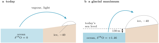
How large is the shift? A mass balance answers it, if the volume of the ice and its mean isotopic composition are known.

Proposition 24.4 (Ice-volume effect by mass balance)

Let the present ocean have mean depth $H$ and a $\delta^{18}$O of 0 (VSMOW). If a layer of sea water of thickness $h$ is removed and stored on land as ice of mean composition $\delta_{\mathrm{ice}}$, the area of the ocean being held fixed, the remaining ocean has

$$\Delta\delta^{18}\mathrm{O}_{\mathrm{sw}} = \frac{-h\,\delta_{\mathrm{ice}}}{H - h}.$$

For small $h$ the shift grows nearly linearly, by $-\delta_{\mathrm{ice}}/H$ per metre of sea level.

Example 24.5 (The last glacial ocean)

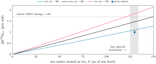
At the Last Glacial Maximum sea level stood 125 to $134\,\mathrm{m}$ below today’s; take $130\,\mathrm{m}$, with $H = 3682.2\,\mathrm{m}$, and ice at $-40$ per mil, the value inferred for the great North American ice sheet. Then $\Delta\delta^{18}\mathrm{O}_{\mathrm{sw}} = 130 \times 40/(3682.2 - 130) = 5200/3552.2 = 1.46$ per mil, about $40/3682.2 = 0.0109$ per mil per metre of sea level. Comparisons of sea-level curves from dated terraces and coral reefs give $0.011$ per mil per metre, in agreement; a scaling of $0.13$ per mil per $10\,\mathrm{m}$, used in some reconstructions, corresponds to ice at about $-50$ per mil. A direct measurement of the change, from the $\delta^{18}$O of the water still held in the pores of glacial sediment, gives $1.0 \pm 0.1$ per mil.

The figure below shows how strongly the answer depends on the composition assumed for the ice. The difference between $1.0$ and $1.5$ per mil is not small: at $0.21$ per mil per degree, it is worth more than two degrees of deep-ocean temperature. The relation is also not quite linear: the ocean that remains shrinks as the ice grows, and the mean $\delta^{18}$O of the ice itself changes as ice sheets of different composition grow and decay. Reconstructions of sea level from $\delta^{18}$O therefore often use a linear relation calibrated on the pore-water value, while recognising that the true relation should be nonlinear.

The benthic stack

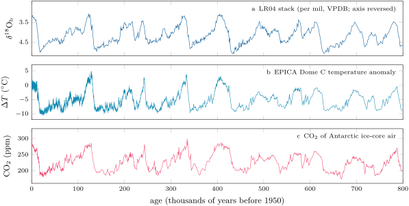
Records of benthic $\delta^{18}$O from many cores, aligned and averaged, form a stack whose noise is lower than that of any single core. The LR04 stack combines 57 records from sites spread over the world ocean and spans 5.3 million years. Between today, $3.23$ per mil, and the mean of $19$ to $23\,\mathrm{ka}$, $4.92$ per mil, it changes by $1.69$ per mil, more than any plausible ice-volume effect. As Shackleton and Opdyke concluded, most of the change is the ice; but a few tenths of a per mil remain for the deep water to have cooled. The problem of this chapter measures that residual.

24.3 Ice cores

The snow that falls on an ice sheet keeps the isotopic composition it had when it fell, and the colder the place and the time, the lighter it is. In Antarctica the annual mean air temperature and the $\delta^{18}$O of the snow follow a strong linear relation from one site to another, with a slope of about $0.8$ per mil per degree, as the Rayleigh distillation of the vapour on its way inland predicts. Hydrogen is used as much as oxygen: on the meteoric water line, $\delta$D varies about eight times as fast as $\delta^{18}$O, and the $\delta$D record of Antarctic ice was chosen for its greater sensitivity to temperature.

A slope measured across space is not necessarily a slope in time. In Greenland, where the ice temperature itself has been reconstructed by other methods, the change of $\delta^{18}$O per degree over time turns out to be 0.3 to $0.6$ per mil, against a present spatial slope of about $0.7$: the seasons of snowfall, the sources of the moisture and its paths changed with the climate. The early Antarctic temperatures were computed with a spatial relation measured in the snow; more recent ones use general circulation models that simulate the water isotopes.

The core of EPICA Dome C, drilled through $3260\,\mathrm{m}$ of ice, reaches $800\,000$ years. Its $\delta$D was measured on samples $55\,\mathrm{cm}$ long, with an accuracy of $0.5$ per mil, and converted to a temperature anomaly relative to the average of the last thousand years, after correcting for the changing composition of the sea water that fed the snow and for the changing elevation of the ice sheet. Between glacial and interglacial times the temperature varied by about $15\,{}^{\circ}\mathrm{C}$. Between the last two thousand years and the Last Glacial Maximum ($19$ to $23\,\mathrm{ka}$), the mean $\delta$D falls from $-396.6$ to $-441.7$ per mil and the anomaly from $-0.09$ to $-9.39\,{}^{\circ}\mathrm{C}$.

Ice also keeps air. The firn, the packed snow of the top tens of metres, is open to the atmosphere until its pores close off at the transition to ice, 50 to $120\,\mathrm{m}$ down; the air in a bubble is therefore younger than the ice around it. Measured in the bubbles, the CO$_2$ of the air was $189.7\,\mathrm{ppm}$ on average between $19$ and $23\,\mathrm{ka}$, and $279.4\,\mathrm{ppm}$ over the two thousand years before industry. The panels (b) and (c) of the figure above rise and fall together over the last $800\,000$ years.

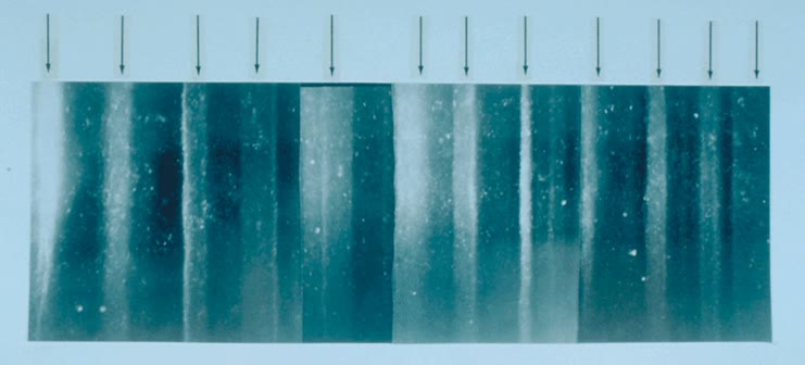
Greenland cores reach only about $120\,000$ years, but the snow accumulates faster there and the record is finer; it shows the abrupt warmings of the last glacial period known as the Dansgaard–Oeschger events. Near the top of a thick core, the seasons themselves can be seen.

In the lab — Cutting an ice core

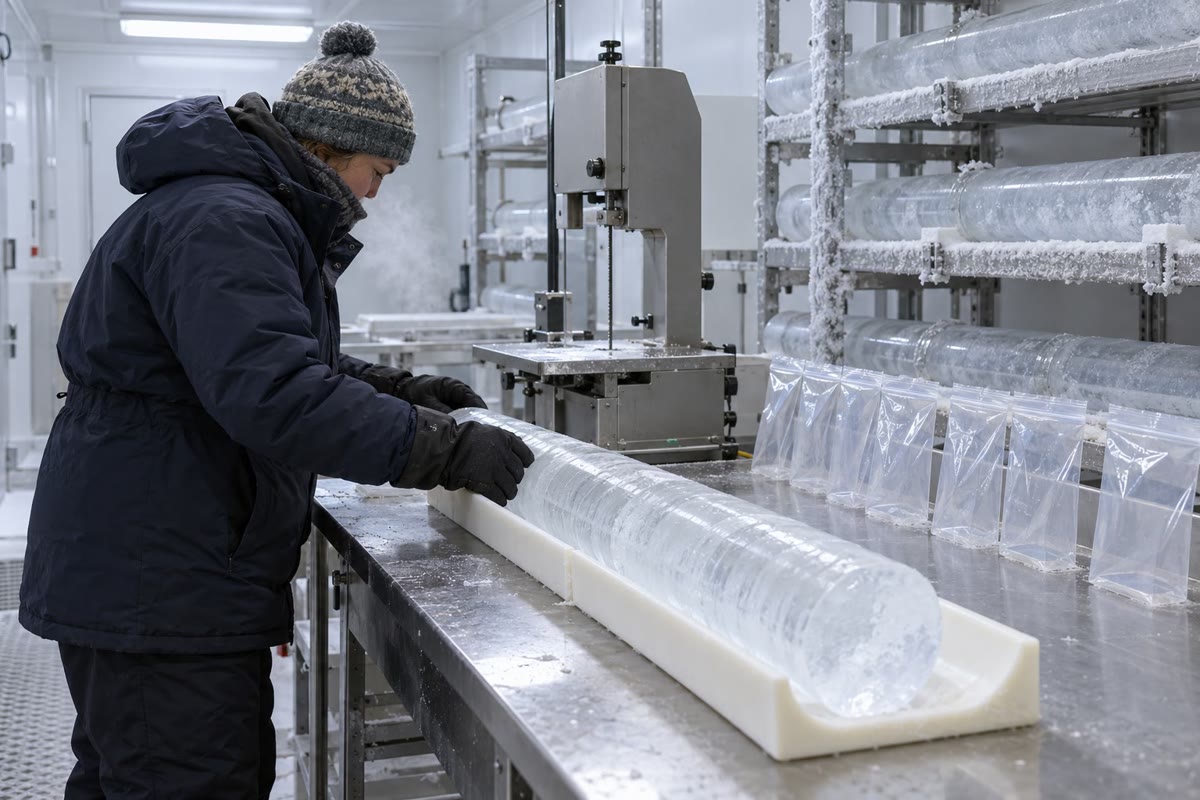
At a national ice-core facility, the cores are kept in tubes, one metre of core per tube, in an archive freezer at $-36\,{}^{\circ}\mathrm{C}$; the scientists work in an examination room at $-24\,{}^{\circ}\mathrm{C}$. When a new core arrives, a core processing line forms: scientists and staff measure, catalogue and cut each section, at typically 30 to $35\,\mathrm{m}$ a day, so that a core $1000\,\mathrm{m}$ long takes six to eight weeks. One researcher shaves the core smooth with a planer and measures its electrical conductivity, a key to defining and dating the layers; another saws the pieces whose trapped air will be analysed for carbon dioxide and methane; the samples are then shipped to the laboratories that measure them. At EPICA Dome C, each sample of the $\delta$D profile was $55\,\mathrm{cm}$ of ice.

24.4 Other proxies, other archives

The magnesium of shells

The calcite of foraminifera takes up a little magnesium in place of calcium, and more of it when the water is warmer. The ratio does not depend on the isotopic composition of the water, so it gives the temperature that the $\delta^{18}$O equation needs.

Definition 24.6 (Mg/Ca ratio (proxy))

The Mg/Ca ratio (proxy) is the ratio of magnesium to calcium in the calcite of foraminiferal shells, in $\mathrm{mmol}/\mathrm{mol}$, used as a measure of the temperature of the water in which the shell grew through an exponential calibration

$$\text{Mg/Ca} = B\,\mathrm{e}^{A T},$$

with $A$ close to $0.09\,/{}^{\circ}\mathrm{C}$ for planktonic species and $B$ specific to the species.

With $A = 0.09$ the ratio grows by $\mathrm{e}^{0.09} - 1 = 9.4\,\%$ per degree, whatever the temperature. For one planktonic species of cold waters, the calibration predicted from temperature alone is $\text{Mg/Ca} = 0.4\,\mathrm{e}^{0.09T}$; a fit to 235 shells from plankton tows and the tops of North Atlantic cores gives $0.372\,\mathrm{e}^{0.0936T}$, with $r^2 = 0.90$. At low temperatures the measured ratios depart from the curve, and the departure is attributed to the concentration of carbonate ion in the sea water: a proxy rarely depends on one variable only. Benthic species are less sensitive, about $0.1\,\mathrm{mmol}/\mathrm{mol}$ per degree for low-magnesium species living in the sediment.

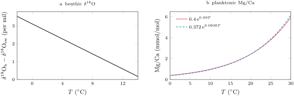
Measured on the same shells, Mg/Ca and $\delta^{18}$O give two equations for two unknowns: Mg/Ca gives $T$, and Proposition 24.2 then gives $\delta^{18}\mathrm{O}_{\mathrm{sw}}$, the ice-volume signal. Applied to benthic shells of the deep North-West Atlantic, the method finds the water of the Last Glacial Maximum only about $2\,{}^{\circ}\mathrm{C}$ colder than today’s ($-1.78 \pm 0.56\,{}^{\circ}\mathrm{C}$), while estimates from pore waters put both deep water masses near freezing in the glacial ocean, $-1.1$ and $-1.9\,{}^{\circ}\mathrm{C}$, where today they are at 2 to $4\,{}^{\circ}\mathrm{C}$ and 0 to $1\,{}^{\circ}\mathrm{C}$.

Tree rings

Definition 24.7 (Dendroclimatology; cross-dating)

Dendroclimatology is the reconstruction of past climate from the annual growth rings of trees: their width, the density of their wood and their isotopic composition. Cross-dating is the matching of the pattern of wide and narrow rings between trees, which assigns to every ring its absolute calendar year and reveals rings that are locally absent in a single tree.

A ring is wider when conditions favour growth. Cross-dating is reliable at climatically extreme sites, where one climate factor limits the growth of all the trees, so that they share the same pattern; it may fail where no single factor dominates, and where many rings are locally absent. Overlapping the patterns of living trees, old timbers and buried wood extends a chronology back year by year; a recent study dated a chronology of 100 subfossil yews of eastern England to the 456 years from 2668 to 2213 BCE, using the $\delta^{18}$O of more than $1500$ of their rings against an absolutely dated oak chronology. The International Tree-Ring Data Bank holds the ring widths, densities, isotopes and chronologies of more than $5000$ sites on six continents.

Caves and lakes

Definition 24.8 (Speleothem; varve)

A speleothem is a mineral deposit formed from groundwater within a cave: stalagmites, stalactites and other forms. A varve is the deposit of one year in a lake or sea floor sediment, usually a pair of laminae of contrasting composition, one laid down in summer and one in the rest of the year.

Speleothems grow layer by layer from the groundwater that reaches a cave; the thickness of their layers and their isotopic records give past climate conditions. Some are annually banded, and some contain compounds that can be dated radiometrically. The time scale of the Greenland cores agrees with that of the speleothems of Hulu Cave to within 800 years over the last $60\,000$ years: two archives, dated by different methods, check each other.

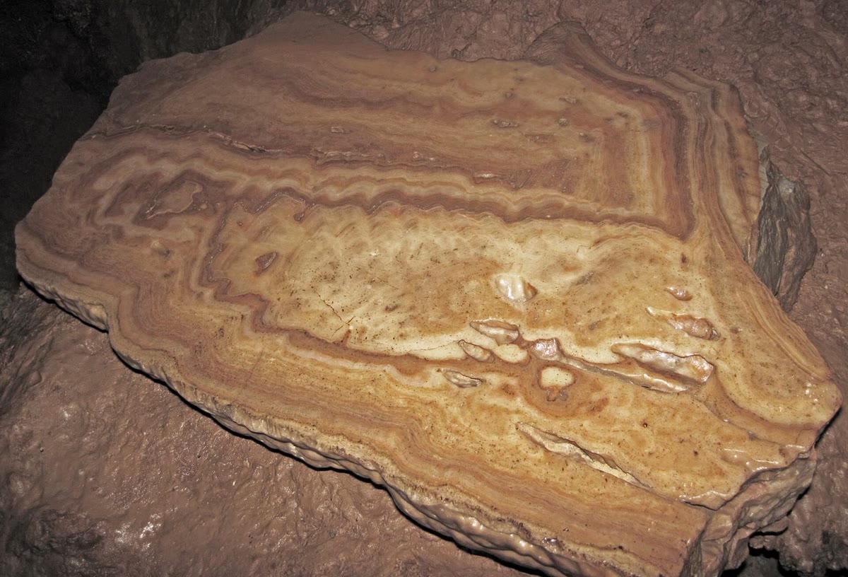
In the deep basin of Crawford Lake, in Ontario, the bottom water, saltier and more alkaline than the water above it, holds no animals large enough to stir the mud, although it is well oxygenated, and every year adds a couplet: a layer of organic matter, capped by the calcite that precipitates each summer from the alkaline surface water. Lake sediments also keep the pollen of the surrounding vegetation, read by pollen analysis; varved or not, they record the land.

24.5 Age models

A proxy without a date is a curiosity. Every archive needs a relation between depth, or ring, or band, and age.

Definition 24.9 (Age model; annual layer counting)

An age model is the function that assigns an age, with its uncertainty, to every depth of an archive. Annual layer counting builds an age model by counting, from the top down, the layers that each record one year (ice layers, varves, bands), each layer whose annual nature is doubtful being counted as half a year plus or minus half a year.

Method 24.10 (Building an age model)

1. Where the archive has annual layers, count them from a known top, recording the uncertain ones separately.
2. Where it has none, or they cannot be resolved, fix tie points: depths dated independently, by radiocarbon or other radiometric methods, by a dated volcanic ash, or by matching a well-dated record.
3. Between tie points, interpolate, linearly in depth if nothing better is known, or with a model of how the archive accumulated and thinned.
4. Carry the uncertainty of each step to every depth.

The Greenland Ice Core Chronology 2005, GICC05, counts annual layers in three Greenland cores, and in the glacial part in the NorthGRIP core alone, over the last $60\,000$ years; its ages are given in years before AD 2000, written b2k. The uncertain layers, counted as $\frac12 \pm \frac12$, add up to the maximum counting error, which the authors regard as two standard deviations. At the start of the Holocene, 11 703 years b2k, it is 50 years; at the onset of the Greenland interstadial 17, $59\,440$ years b2k, it is $1287$ years.

Proposition 24.11 (Growth of a counting error)

Let a count contain $n$ uncertain layers, each counted as $\frac12$ with an error of standard deviation $\frac12$. If the errors of the layers are independent, the standard deviation of the total is $\frac12\sqrt{n}$; if they are all of the same sign, the error of the total is $\frac12 n$.

At GI-17, the $1287$ years of maximum counting error mean $2574$ uncertain layers. Were their errors independent, the total would be uncertain by only $\frac12\sqrt{2574} = 25$ years. The linear sum is the cautious choice: the doubtful layers of one stretch of ice are judged by the same counters with the same criteria, and there is no reason to expect their errors to cancel. The older part of the record was counted independently by two of the authors; their counts differ by less than the absolute error, though locally by more than the final counting error. The maximum counting error averages about $1\,\%$ of the time a section spans in the Holocene and $5\,\%$ in the glacial part.

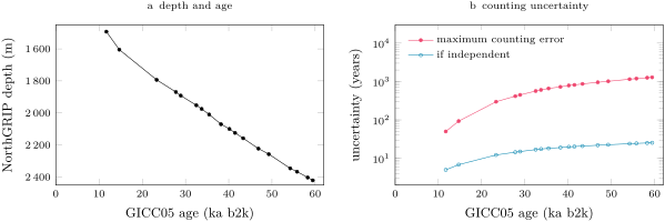
Annual layers thin with depth, because the ice flows and spreads as it sinks: between the start of the Holocene and GI-1, the mean layer is $3.75\,\mathrm{cm}$ thick in NorthGRIP; between GI-16 and GI-17, $1.54\,\mathrm{cm}$; around $100\,\mathrm{ka}$, flow models put it near $1\,\mathrm{cm}$. The thinner the layers, the harder they are to tell apart.

24.6 Calibration

Every number read from a proxy comes through a calibration.

Definition 24.12 (Proxy calibration)

A proxy calibration is the empirical or theoretical relation that converts the value of a proxy into the climate variable it stands for, established on samples for which both are known, together with its uncertainty and the range of conditions over which it is valid.

The samples for which both are known are modern: shells caught in plankton tows, the tops of sediment cores compared with the water above them, recent snow compared with the temperature of its site, the outer rings of trees compared with the records of a weather station. The relation is then fitted by least squares; for an exponential law such as the Mg/Ca calibration the fit is made on the logarithm, which turns $\text{Mg/Ca} = B\,\mathrm{e}^{AT}$ into the straight line $\ln(\text{Mg/Ca}) = \ln B + AT$. A calibration is validated on samples that were not used to fit it: part of the modern data is put aside and predicted.

Three limits remain. A calibration measured across space, from place to place today, may not hold in time, as the Greenland ice has shown. A calibration measured over today’s range of conditions must be extrapolated with care: the Mg/Ca of shells departs from its law at low temperatures, where another variable, the carbonate ion, takes over. And a relation that is linear over a small range may not be linear over a large one, as the ice-volume effect is not. The method of this chapter answers them in the same way: measure two independent proxies on the same sample, and let each check the other.

Exercises

Data for the exercises, unless stated otherwise: mean ocean depth $H = 3682.2\,\mathrm{m}$, ocean area $361.84 \times 10^{6}\,\mathrm{km}^{2}$; the benthic calibration of Proposition 24.2; the planktonic calibration $\text{Mg/Ca} = 0.4\,\mathrm{e}^{0.09T}$ ($\mathrm{mmol}/\mathrm{mol}$, ${}^{\circ}\mathrm{C}$); $\delta$ values of waters and ice in per mil VSMOW, of calcite in per mil VPDB.

Exercise 24.1 ★

Today the continental ice holds about $27.5 \times 10^{6}\,\mathrm{km}^{3}$ and the ocean $1350 \times 10^{6}\,\mathrm{km}^{3}$ of water (take the volumes as amounts of water). (a) If the ice has a mean $\delta^{18}$O of $-30$ per mil and the ocean 0, what is the $\delta^{18}$O of the whole hydrosphere, neglecting the fresh water? (b) If all the ice melted, what would the $\delta^{18}$O of the ocean become? (c) What fraction of the water is ice?

Solution

Solution of Exercise 24.1.

(a) $\delta = (27.5 \times (-30) + 1350 \times 0)/(1350 + 27.5) = -825/1377.5 = -0.60$ per mil. (b) The ocean would then hold all the water: $-0.60$ per mil, $0.60$ per mil lighter than today. (c) $27.5/1377.5 = 2.0\,\%$.

Exercise 24.2 ★

A benthic shell has $\delta^{18}\mathrm{O}_{\mathrm{b}} = 2.50$ per mil. (a) Compute its temperature if the sea water had $\delta^{18}\mathrm{O}_{\mathrm{sw}} = 0$. (b) Compute it if the sea water had $+1.0$ per mil. (c) Another shell, from the same water at $0$ per mil, has $2.71$ per mil: by how much was its water colder?

Solution

Solution of Exercise 24.2.

(a) $T = 16.1 - 4.76\,(2.50 - (0 - 0.27)) = 16.1 - 4.76 \times 2.77 = 16.1 - 13.19 = 2.9\,{}^{\circ}\mathrm{C}$. (b) $T = 16.1 - 4.76\,(2.50 - 0.73) = 16.1 - 8.43 = 7.7\,{}^{\circ}\mathrm{C}$: the same shell gives a temperature almost five degrees higher if the water was heavier, which is why the composition of the water must be known. (c) The shell is $2.71 - 2.50 = 0.21$ per mil heavier, so its water was $4.76 \times 0.21 = 1.0\,{}^{\circ}\mathrm{C}$ colder, at $1.9\,{}^{\circ}\mathrm{C}$.

Exercise 24.3 ★

(a) Compute the Mg/Ca ratio of the planktonic calibration at $10\,{}^{\circ}\mathrm{C}$ and at $20\,{}^{\circ}\mathrm{C}$. (b) By what factor does the ratio grow over these ten degrees, and by what percentage per degree? (c) Compute the temperature of shells with Mg/Ca = 2.0 and $1.0\,\mathrm{mmol}/\mathrm{mol}$.

Solution

Solution of Exercise 24.3.

(a) $0.4\,\mathrm{e}^{0.9} = 0.98\,\mathrm{mmol}/\mathrm{mol}$ and $0.4\,\mathrm{e}^{1.8} = 2.42\,\mathrm{mmol}/\mathrm{mol}$. (b) The factor is $\mathrm{e}^{0.9} = 2.46$; per degree $\mathrm{e}^{0.09} = 1.094$, a growth of $9.4\,\%$ per degree. (c) $T = \ln(\text{Mg/Ca}/0.4)/0.09$: $\ln 5/0.09 = 17.9\,{}^{\circ}\mathrm{C}$ and $\ln 2.5/0.09 = 10.2\,{}^{\circ}\mathrm{C}$.

Exercise 24.4 ★

A chronology of subfossil yews runs from 2668 to 2213 BCE. (a) How many years does it cover, counting both end years? (b) Why does a chronology built from many trees deserve more trust than the count of the rings of a single tree? (c) Why would you expect cross-dating to be easier for trees near the cold tree line than for trees in a mild, moist lowland forest?

Solution

Solution of Exercise 24.4.

(a) $2668 - 2213 + 1 = 456$ years. (b) A single tree may lack a ring locally, or show a ring that cannot be read; matching the patterns of wide and narrow rings across many trees reveals the missing rings and fixes the year of every ring, and the agreement between trees measures the reliability of the dating. (c) At the tree line one factor, the cold of the growing season, limits all the trees, so they share the same pattern of good and bad years; in a mild, moist lowland no single factor dominates, the patterns of the trees differ, and cross-dating may fail.

Exercise 24.5 ★★

(a) With Proposition 24.4, compute the ice-volume effect for a sea-level fall of $125\,\mathrm{m}$ and of $134\,\mathrm{m}$, with ice at $-40$ per mil. (b) Compute it for $130\,\mathrm{m}$ with ice at $-30$, $-35$ and $-50$ per mil. (c) Which mean composition of the ice would make the effect of a $130\,\mathrm{m}$ fall equal to the $1.0$ per mil measured in pore waters? Compare with the compositions of the present ice sheets.

Solution

Solution of Exercise 24.5.

(a) $125 \times 40/(3682.2 - 125) = 5000/3557.2 = 1.41$ per mil; $134 \times 40/3548.2 = 5360/3548.2 = 1.51$ per mil. (b) With $H - h = 3552.2$: $3900/3552.2 = 1.10$, $4550/3552.2 = 1.28$ and $6500/3552.2 = 1.83$ per mil. (c) $\delta_{\mathrm{ice}} = -1.0 \times 3552.2/130 = -27.3$ per mil, heavier than any present ice sheet (Greenland $-30$ to $-35$, the North American ice sheet $-40$, Antarctic ice as low as $-50$). The mass balance with realistic ice and the pore-water measurement do not agree; the gap of about half a per mil is a real uncertainty of the method.

Exercise 24.6 ★★

Compare the two calibrations of the Mg/Ca of the same planktonic species: the one predicted from temperature alone, $0.4\,\mathrm{e}^{0.09T}$, and the fit $0.372\,\mathrm{e}^{0.0936T}$. (a) At what temperature do they agree? (b) At $2\,{}^{\circ}\mathrm{C}$, by what percentage is the fitted ratio lower than the predicted one? (c) A shell grown at $2\,{}^{\circ}\mathrm{C}$ follows the fitted law; what temperature would the predicted law give for it?

Solution

Solution of Exercise 24.6.

(a) $0.372\,\mathrm{e}^{0.0936T} = 0.4\,\mathrm{e}^{0.09T}$ gives $\mathrm{e}^{0.0036T} = 0.4/0.372 = 1.0753$, so $T = \ln 1.0753/0.0036 = 20.2\,{}^{\circ}\mathrm{C}$. (b) At $2\,{}^{\circ}\mathrm{C}$: $0.4\,\mathrm{e}^{0.18} = 0.479$ and $0.372\,\mathrm{e}^{0.1872} = 0.449$, so the fitted ratio is $0.449/0.479 = 0.937$, $6.3\,\%$ lower. (c) $T = \ln(0.449/0.4)/0.09 = \ln 1.1225/0.09 = 1.3\,{}^{\circ}\mathrm{C}$: the predicted law reads the shell about $0.7\,{}^{\circ}\mathrm{C}$ too cold. In cold water the choice of calibration matters at the level of a degree.

Exercise 24.7 ★★

In the NorthGRIP core, the start of the Holocene lies at $1492.45\,\mathrm{m}$ and $11\,703$ years b2k, the onset of GI-1 at $1604.64\,\mathrm{m}$ and $14\,692$ years; the onset of GI-16 at $2402.55\,\mathrm{m}$ and $58\,280$ years, that of GI-17 at $2420.44\,\mathrm{m}$ and $59\,440$ years. (a) Compute the mean thickness of the annual layers in each interval. (b) Why are they thinner deeper down? (c) Why does annual layer counting become impossible at some depth?

Solution

Solution of Exercise 24.7.

(a) From the Holocene to GI-1, $112.19\,\mathrm{m}$ of ice for 2989 years: $11\,219/2989 = 3.75\,\mathrm{cm}$ per year; from GI-16 to GI-17, $17.89\,\mathrm{m}$ for 1160 years: $1789/1160 = 1.54\,\mathrm{cm}$ per year. (b) The ice flows: as each layer is buried it spreads sideways and thins, and the deeper, older layers have been thinned longer. (c) When the layers become too thin, a centimetre or less, the instruments can no longer resolve one year from the next, and the age model must use tie points or flow models instead.

Exercise 24.8 ★★

Use the first two tie points of Exercise 24.7, with maximum counting errors of 50 and 93 years. (a) By linear interpolation in depth, give the age of the ice at $1550\,\mathrm{m}$. (b) Express it in years before 1950. (c) Interpolate the uncertainty in the same way.

Solution

Solution of Exercise 24.8.

(a) The fraction of the interval is $(1550 - 1492.45)/(1604.64 - 1492.45) = 57.55/112.19 = 0.513$, so the age is $11\,703 + 0.513 \times 2989 = 11\,703 + 1533 = 13\,236$ years b2k. (b) 1950 is 50 years before 2000: $13\,186$ years before 1950. (c) $50 + 0.513 \times (93 - 50) = 72$ years.

Exercise 24.9 ★★

The maximum counting error of GICC05 is 93 years at GI-1 and $1287$ years at GI-17. (a) How many uncertain layers does each represent? (b) What would the uncertainty be if the errors of these layers were independent, each of standard deviation half a year? (c) By what factor does the linear sum exceed the independent estimate in each case, and why does the factor grow with depth?

Solution

Solution of Exercise 24.9.

(a) Each uncertain layer contributes half a year: $2 \times 93 = 186$ and $2 \times 1287 = 2574$ uncertain layers. (b) $\frac12\sqrt{186} = 6.8$ years and $\frac12\sqrt{2574} = 25.4$ years. (c) $93/6.8 = 14$ and $1287/25.4 = 51$. The ratio of $\frac12 n$ to $\frac12\sqrt{n}$ is $\sqrt{n}$: it grows as the square root of the number of uncertain layers, so the choice between the two rules matters more and more with depth.

Exercise 24.10 ★★★

At EPICA Dome C the mean $\delta$D of the ice is $-396.6$ per mil over the last two thousand years and $-441.7$ per mil over 19 to $23\,\mathrm{ka}$. (a) The Antarctic spatial slope of $\delta^{18}$O is $0.8$ per mil per degree. With the meteoric water line, convert it to a slope of $\delta$D and estimate the glacial cooling. (b) The glacial ocean was $1.0$ per mil heavier in $\delta^{18}$O, so the snow formed from it was heavier too. Assuming the $\delta$D of the ocean changed eight times as much, correct the glacial $\delta$D and estimate the cooling again. (c) The published anomaly is $-0.09$ and $-9.39\,{}^{\circ}\mathrm{C}$ for the two periods; what slope of $\delta$D per degree does that imply, and what other correction does the published series contain?

Solution

Solution of Exercise 24.10.

(a) On the meteoric water line $\delta$D changes eight times as much as $\delta^{18}$O, so the slope is $8 \times 0.8 = 6.4$ per mil of $\delta$D per degree. The drop is $441.7 - 396.6 = 45.1$ per mil, hence a cooling of $45.1/6.4 = 7.0\,{}^{\circ}\mathrm{C}$. (b) The glacial ocean was about $8 \times 1.0 = 8$ per mil heavier in $\delta$D; snow formed from today’s ocean would have been lighter by as much, $-441.7 - 8 = -449.7$ per mil. The drop becomes $53.1$ per mil and the cooling $53.1/6.4 = 8.3\,{}^{\circ}\mathrm{C}$. (c) $9.39 - 0.09 = 9.30\,{}^{\circ}\mathrm{C}$, so $45.1/9.30 = 4.85$ per mil per degree. The published series is also corrected for the changing elevation of the ice sheet, and its temperature relation comes from models that simulate the water isotopes, not from the spatial slope alone.

Exercise 24.11 ★★★

A calibration of the Mg/Ca of a planktonic species uses six core-top samples (water temperature, Mg/Ca in $\mathrm{mmol}/\mathrm{mol}$): (4, 0.59), (8, 0.80), (12, 1.21), (16, 1.65), (20, 2.47), (24, 3.41). (a) Fit $\ln(\text{Mg/Ca}) = \ln B + AT$ by least squares, and give $A$ and $B$. (b) Compute the residuals of the logarithm, and compare the fit with the law $0.4\,\mathrm{e}^{0.09T}$. (c) Give the temperature of a glacial shell with Mg/Ca = 1.30. (d) A shell has Mg/Ca = 0.45: compute its temperature, and say why this value deserves less trust than the previous one.

Solution

Solution of Exercise 24.11.

(a) The logarithms of the ratios are $-0.528$, $-0.223$, $0.191$, $0.501$, $0.904$, $1.227$; their mean is $0.345$ and the mean temperature 14. With $S_{TT} = \sum (T - 14)^2 = 280$ and $S_{T\ell} = \sum (T - 14)(\ell - 0.345) = 24.93$, $A = 24.93/280 = 0.0890\,/{}^{\circ}\mathrm{C}$ and $\ln B = 0.345 - 0.0890 \times 14 = -0.901$, so $B = 0.406\,\mathrm{mmol}/\mathrm{mol}$. (b) The residuals are $+0.017$, $-0.034$, $+0.023$, $-0.023$, $+0.025$ and $-0.009$, a few per cent of the ratio, with no trend; the fit is close to $0.4\,\mathrm{e}^{0.09T}$. (c) $T = (\ln 1.30 + 0.901)/0.0890 = (0.262 + 0.901)/0.0890 = 13.1\,{}^{\circ}\mathrm{C}$. (d) $T = (\ln 0.45 + 0.901)/0.0890 = (-0.799 + 0.901)/0.0890 = 1.2\,{}^{\circ}\mathrm{C}$. This value lies below the coldest sample of the calibration, $4\,{}^{\circ}\mathrm{C}$: the law is extrapolated, and at low temperatures the Mg/Ca of shells is known to depart from the exponential law under the influence of the carbonate ion.

Exercise 24.12 ★★★

An ice sheet grows in two stages: first $60\,\mathrm{m}$ of sea level is stored as ice at $-30$ per mil, then $70\,\mathrm{m}$ more as ice at $-45$ per mil. (a) Show that the mass balance of Proposition 24.4 becomes $(H - h)\,\Delta\delta = -\sum_i h_i\delta_i$ for several stores of ice, and compute the ice-volume effect after each stage. (b) What is the mean composition of the ice at the end? (c) A linear rule, calibrated on the end state, converts $\Delta\delta$ into sea level. What sea-level fall would it infer for the first stage, and why does it err?

Solution

Solution of Exercise 24.12.

(a) Per unit of ocean area, the water of the present ocean, $H$ at 0, is shared between the stores $h_i$ at $\delta_i$ and the remaining ocean $H - h$, with $h = \sum h_i$: $0 = \sum h_i\delta_i + (H - h)\,\Delta\delta$. After the first stage $\Delta\delta = 60 \times 30/(3682.2 - 60) = 1800/3622.2 = 0.50$ per mil; after the second $(1800 + 70 \times 45)/(3682.2 - 130) = 4950/3552.2 = 1.39$ per mil. (b) $-4950/130 = -38.1$ per mil. (c) The rule is $1.39/130 = 0.0107$ per mil per metre, and gives $0.50/0.0107 = 47\,\mathrm{m}$ for the first stage instead of $60\,\mathrm{m}$: the first ice was heavier than the mean, so each of its metres shifted the ocean less. A linear rule calibrated on one state misreads the others when the mean composition of the ice changes.

Problem 24.1

Weekend problem — One shell, two signals

How much colder was the deep ocean at the Last Glacial Maximum? The $\delta^{18}$O of benthic shells mixes the answer with the volume of the ice; this problem separates the two. Use the data of the exercises; sea level stood 125 to $134\,\mathrm{m}$ below today’s, and the ice of the North American ice sheet is thought to have had a $\delta^{18}$O of about $-40$ per mil.

Part I — The ice on land.

1. Compute the volume of water removed from the ocean by a sea-level fall of $130\,\mathrm{m}$.
2. Compute the ice-volume effect of that fall with ice at $-40$ per mil.
3. Compute it for falls of $125\,\mathrm{m}$ and $134\,\mathrm{m}$.
4. Compute it for $130\,\mathrm{m}$ with ice at $-35$ and at $-50$ per mil. Which uncertainty matters more, that of the sea level or that of the ice?
5. The pore waters of glacial sediments give $1.0 \pm 0.1$ per mil. What mean composition of the ice would a fall of $130\,\mathrm{m}$ require to produce it?
6. Compute the shift per metre of sea level for small falls with ice at $-40$ per mil, and compare with the value of $0.011$ per mil per metre derived from dated sea levels.

Part II — Two thermometers.

7. Show from Proposition 24.2 that a cooling of $1\,{}^{\circ}\mathrm{C}$ at constant water composition raises $\delta^{18}\mathrm{O}_{\mathrm{b}}$ by $0.21$ per mil.
8. Compute $\delta^{18}\mathrm{O}_{\mathrm{b}}$ of a benthic shell grown today in water at $2.0\,{}^{\circ}\mathrm{C}$ with $\delta^{18}\mathrm{O}_{\mathrm{sw}} = 0$.
9. Compute it for a glacial shell grown in water at $-1.0\,{}^{\circ}\mathrm{C}$ with $\delta^{18}\mathrm{O}_{\mathrm{sw}} = +1.0$ per mil. What is the change between the two shells, and how much of it is due to the water’s composition?
10. A planktonic shell has Mg/Ca = $2.0\,\mathrm{mmol}/\mathrm{mol}$. Compute its temperature.
11. Low-magnesium benthic shells gain about $0.1\,\mathrm{mmol}/\mathrm{mol}$ per degree. A glacial shell has a Mg/Ca $0.18\,\mathrm{mmol}/\mathrm{mol}$ lower than a modern one of the same species from the same place. What cooling does that indicate?
12. Why does Mg/Ca give a temperature that does not depend on the volume of ice?

Part III — The residual. The LR04 stack reads $3.23$ per mil today and $4.92$ per mil on average over 19 to $23\,\mathrm{ka}$.

13. Compute the change of the stack between today and the Last Glacial Maximum.
14. If all of it were ice-volume effect, with ice at $-40$ per mil, what sea-level fall would it imply (invert Proposition 24.4)? Is that consistent with the sea-level evidence?
15. Take the ice-volume effect of question 2. What residual remains for the temperature, and what cooling of the deep water does it give?
16. Take instead the pore-water value, $1.0$ per mil. What residual and what cooling?
17. Another reconstruction uses $0.25$ per mil per degree. Repeat the two estimates with it.
18. Today the North Atlantic Deep Water is at 2 to $4\,{}^{\circ}\mathrm{C}$ and the Antarctic Bottom Water at 0 to $1\,{}^{\circ}\mathrm{C}$; pore waters put them at $-1.1$ and $-1.9\,{}^{\circ}\mathrm{C}$ in the glacial ocean, and the Mg/Ca of benthic shells finds the deep North-West Atlantic only about $1.8\,{}^{\circ}\mathrm{C}$ colder. What range of cooling do these give, and which of the two estimates of questions 15 and 16 do they favour?

Part IV — The view from the ice. At EPICA Dome C the mean $\delta$D is $-396.6$ per mil over the last two thousand years and $-441.7$ per mil over 19 to $23\,\mathrm{ka}$; the published temperature anomaly is $-0.09$ and $-9.39\,{}^{\circ}\mathrm{C}$.

19. Compute the change of $\delta$D.
20. With a $\delta^{18}$O slope of $0.8$ per mil per degree and the meteoric water line, estimate the cooling at Dome C.
21. Compute the published cooling, and the slope of $\delta$D per degree it implies.
22. The global mean surface was 5 to $7\,{}^{\circ}\mathrm{C}$ colder at the Last Glacial Maximum. Rank the coolings of Dome C, of the globe and of the deep ocean.
23. Why can the deep ocean not have cooled by as much as the surface of Antarctica?
24. To sum up: with the pore-water correction for ice volume, by how much was the deep ocean colder at the Last Glacial Maximum than today?

Solution

Solution of Problem 24.1.

1. $361.84 \times 10^6\ \mathrm{km}^{2} \times 0.130\,\mathrm{km} = 4.70 \times 10^{7}\,\mathrm{km}^{3}$, about 47 million cubic kilometres. 2. $130 \times 40/(3682.2 - 130) = 5200/3552.2 = 1.46$ per mil. 3. $5000/3557.2 = 1.41$ and $5360/3548.2 = 1.51$ per mil. 4. $4550/3552.2 = 1.28$ and $6500/3552.2 = 1.83$ per mil. The composition of the ice moves the answer by $0.55$ per mil, the sea level by $0.10$: the ice matters more. 5. $\delta_{\mathrm{ice}} = -1.0 \times 3552.2/130 = -27.3$ per mil. 6. $40/3682.2 = 0.0109$ per mil per metre, which rounds to the $0.011$ of the dated sea levels. 7. At constant $\delta^{18}\mathrm{O}_{\mathrm{sw}}$, $\mathrm{d}T = -4.76\,\mathrm{d}\delta^{18} \mathrm{O}_{\mathrm{b}}$, so $\mathrm{d}T = -1$ gives $\mathrm{d}\delta^{18}\mathrm{O}_{\mathrm{b}} = 1/4.76 = 0.21$ per mil. 8. $\delta^{18}\mathrm{O}_{\mathrm{b}} = (16.1 - T)/4.76 + \delta^{18}\mathrm{O}_{\mathrm{sw}} - 0.27 = 14.1/4.76 - 0.27 = 2.96 - 0.27 = 2.69$ per mil. 9. $17.1/4.76 + 1.0 - 0.27 = 3.59 + 0.73 = 4.32$ per mil. The change is $4.32 - 2.69 = 1.63$ per mil: $1.00$ from the water and $3.0 \times 0.21 = 0.63$ from the cooling of $3\,{}^{\circ}\mathrm{C}$. 10. $T = \ln(2.0/0.4)/0.09 = \ln 5/0.09 = 17.9\,{}^{\circ}\mathrm{C}$. 11. $0.18/0.1 = 1.8\,{}^{\circ}\mathrm{C}$ of cooling. 12. Mg/Ca is a ratio of two elements in the calcite, set by the temperature of calcification; it does not involve the isotopes of oxygen, and so it ignores the composition of the water that the ice changes. 13. $4.92 - 3.23 = 1.69$ per mil. 14. Solving $\Delta = h \times 40/(H - h)$ for $h$: $h = H\Delta/(\Delta + 40) = 3682.2 \times 1.69/41.69 = 149\,\mathrm{m}$, more than the 125 to $134\,\mathrm{m}$ of the sea-level evidence: part of the change must be cooling. 15. $1.69 - 1.46 = 0.23$ per mil, and $4.76 \times 0.23 = 1.1\,{}^{\circ}\mathrm{C}$. 16. $1.69 - 1.00 = 0.69$ per mil, and $4.76 \times 0.69 = 3.3\,{}^{\circ}\mathrm{C}$ (3.28). 17. $0.23/0.25 = 0.9\,{}^{\circ}\mathrm{C}$ and $0.69/0.25 = 2.8\,{}^{\circ}\mathrm{C}$. 18. The North Atlantic Deep Water cooled from 2–$4\,{}^{\circ}\mathrm{C}$ to $-1.1\,{}^{\circ}\mathrm{C}$, by 3.1 to $5.1\,{}^{\circ}\mathrm{C}$; the Antarctic Bottom Water from 0–$1\,{}^{\circ}\mathrm{C}$ to $-1.9\,{}^{\circ}\mathrm{C}$, by 1.9 to $2.9\,{}^{\circ}\mathrm{C}$; the Mg/Ca of the North-West Atlantic gives $1.8\,{}^{\circ}\mathrm{C}$. All lie between about 2 and $5\,{}^{\circ}\mathrm{C}$, around the 2.8 to $3.3\,{}^{\circ}\mathrm{C}$ of the pore-water correction, and above the $1\,{}^{\circ}\mathrm{C}$ of the mass balance with ice at $-40$ per mil. 19. $-396.6 - (-441.7) = 45.1$ per mil. 20. $8 \times 0.8 = 6.4$ per mil per degree, so $45.1/6.4 = 7.0\,{}^{\circ}\mathrm{C}$. 21. $9.39 - 0.09 = 9.30\,{}^{\circ}\mathrm{C}$, and $45.1/9.30 = 4.85$ per mil per degree. 22. Dome C, $9.3\,{}^{\circ}\mathrm{C}$, more than the global surface, 5 to $7\,{}^{\circ}\mathrm{C}$, more than the deep ocean, about $3\,{}^{\circ}\mathrm{C}$. 23. The deep water is already cold today, 0 to $4\,{}^{\circ}\mathrm{C}$, and sea water cannot cool much below its freezing point, which the glacial bottom water nearly reached at $-1.9\,{}^{\circ}\mathrm{C}$: the deep ocean had only a few degrees to lose, while the air over Antarctica has no such floor. 24. With the pore-water correction, the deep ocean was about $3.3\,{}^{\circ}\mathrm{C}$ colder at the Last Glacial Maximum than today, close to the 2 to $5\,{}^{\circ}\mathrm{C}$ of the independent deep-water estimates.