University Chemistry — Year 2 · Bachelor Year 2

13Atomic Orbitals: Shapes, Energies and Sizes

A hydrogen atom has no edge: its electron may be found at any distance from the nucleus, with a probability that falls off quickly but never reaches zero. Yet atoms have sizes, and a sodium atom is about twice as wide as a chlorine atom, though it holds fewer electrons. The Year 1 volume named the states of an electron by three quantum numbers; here each of them becomes a function of position, with a shape, nodes, signs and a size, and a simple set of rules turns them into orbital energies for any atom. These shapes and signs are what the next four chapters combine into molecular orbitals.

You already know

The Year 1 volume: quantum numbers $n$ , $l$ , $m_l$ , $m_s$ ; atomic orbitals as the states $(n, l, m_l)$ ; shells and subshells; screening and effective nuclear charge (qualitatively); electron configurations; the levels of hydrogen, $-E_R/n^2$ with $E_R = 13.6\,\mathrm{eV}$ . From physics: the wavefunction, whose squared modulus is a probability density.

13.1 The wavefunctions of the hydrogen atom

Definition 13.1 (Wavefunction)

The state of an electron is described by a wavefunction $\psi(x, y, z)$ ; $|\psi|^2$ is its probability density: the probability of finding the electron in a small volume $dV$ around a point is $|\psi|^2\,dV$ , and $\int|\psi|^2\,dV = 1$ over all space (the function is normalised). An atomic orbital is the wavefunction of one electron in an atom.

Definition 13.2 (Radial and angular parts)

In spherical coordinates $(r, \theta, \varphi)$ about the nucleus, the orbitals of a hydrogen-like atom factorise as $\psi_{nlm}(r, \theta, \varphi) = R_{nl}(r)\, Y_{lm}(\theta, \varphi)$ : the radial part $R_{nl}$ depends on $n$ and $l$ , the angular part $Y_{lm}$ on $l$ and $m_l$ only.

Theorem 13.3 (The hydrogen-like orbitals)

For a one-electron atom of nuclear charge $Ze$ , with $\rho = Zr/a_0$ and $a_0 = 52.9\,\mathrm{pm}$ the Bohr radius, the radial parts for $n \leq 3$ are, in units of $(Z/a_0)^{3/2}$ :

\begin{array}{ll} R_{1s} = 2\,\mathrm e^{-\rho} & R_{2s} = \dfrac{1}{2\sqrt2}\,(2 - \rho)\,\mathrm e^{-\rho/2} \\[2ex] R_{2p} = \dfrac{1}{2\sqrt6}\,\rho\,\mathrm e^{-\rho/2} & R_{3s} = \dfrac{2}{81\sqrt3}\,(27 - 18\rho + 2\rho^2)\,\mathrm e^{-\rho/3} \\[2ex] R_{3p} = \dfrac{4}{81\sqrt6}\,(6\rho - \rho^2)\,\mathrm e^{-\rho/3} & R_{3d} = \dfrac{4}{81\sqrt{30}}\,\rho^2\,\mathrm e^{-\rho/3} \end{array}

and the real angular parts are $Y_s = 1/\sqrt{4\pi}$ ; $Y_{p_x}, Y_{p_y}, Y_{p_z} = \sqrt{3/(4\pi)}\,(x, y, z)/r$ ; $Y_{d_{xy}} = \sqrt{15/(4\pi)}\,xy/r^2$ (and likewise $xz$ , $yz$ ), $Y_{d_{x^2-y^2}} = \sqrt{15/(16\pi)}\,(x^2 - y^2)/r^2$ , $Y_{d_{z^2}} = \sqrt{5/(16\pi)}\,(3z^2 - r^2)/r^2$ . Their energies are $E_n = -Z^2E_R/n^2$ .

Proof. Admitted at this level. ∎

These functions are the solutions of the Schrödinger equation for one electron and one nucleus, found in the Year 3 volume. The real $p$ and $d$ functions are combinations of the complex ones labelled by $m_l$ ; they point along the axes and are those used to build bonds.

Erwin Schrödinger, who in 1926 wrote the wave equation whose solutions for the hydrogen atom are the orbitals of this chapter, and recovered from them the energy levels that Bohr had postulated. He shared the Nobel Prize in Physics in 1933. (Photograph: Nobel Foundation, public domain, Wikimedia Commons.)

13.2 The radial part

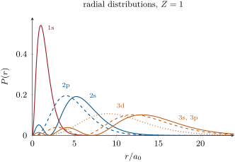
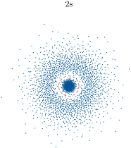
The probability of finding the electron between the spheres of radii $r$ and $r + dr$ is $|\psi|^2$ integrated over the shell of volume $4\pi r^2\,dr$ ; for any orbital, once the angles are integrated out, it is $r^2R^2\,dr$ .

Definition 13.4 (Radial distribution)

The radial distribution function of an orbital is $P(r) = r^2R_{nl}(r)^2$ : $P(r)\,dr$ is the probability that the electron lies between $r$ and $r + dr$ from the nucleus. The most probable radius is the value of $r$ at its largest maximum.

Proposition 13.5 (Normalisation of 1s)

$\int_0^\infty P_{1s}(r)\,dr = 1$ .

Proof. With $Z = 1$ and $r$ in units of $a_0$ , $P_{1s} = 4r^2\mathrm e^{-2r}$ . By parts twice, $\int_0^\infty r^2\mathrm e^{-2r}\,dr = \frac22\int_0^\infty r\,\mathrm e^{-2r}\,dr = \frac12\int_0^\infty\mathrm e^{-2r}\,dr = \frac14$ , and $4 \times \frac14 = 1$ . ∎

Proposition 13.6 (Most probable radius)

For the 1s orbital the most probable radius is $a_0/Z$ . For an orbital with $l = n - 1$ (1s, 2p, 3d, …), it is $n^2a_0/Z$ .

Proof. For $l = n - 1$ the radial part has no node: $R \propto \rho^{n-1}\mathrm e^{-\rho/n}$ , so $P \propto \rho^{2n}\mathrm e^{-2\rho/n}$ and $d\ln P/d\rho = 2n/\rho - 2/n$ , zero for $\rho = n^2$ , that is $r = n^2a_0/Z$ . With $n = 1$ , $r = a_0/Z$ . ∎

Proposition 13.7 (Mean radius of 1s)

The mean distance of a 1s electron from the nucleus is $\langle r\rangle = 3a_0/(2Z)$ , larger than its most probable radius.

Proof. With $Z = 1$ : $\langle r\rangle = \int_0^\infty r\,P(r)\,dr = 4\int_0^\infty r^3\mathrm e^{-2r} \,dr = 4 \times 3!/2^4 = 3/2$ . The distribution has a long tail at large $r$ , which pulls the mean beyond the maximum. ∎

Definition 13.8 (Nodes)

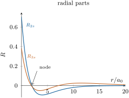
A nodal surface of an orbital is a surface on which the wavefunction is zero and changes sign. It is a radial node (a sphere) when the radial part vanishes, an angular node (a plane or a cone through the nucleus) when the angular part does.

Proposition 13.9 (Counting nodes)

An orbital $(n, l)$ has $n - l - 1$ radial nodes and $l$ angular nodes, $n - 1$ in all.

Proof. On the functions of Theorem 13.3: $R_{2s}$ vanishes at $\rho = 2$ , $R_{3s}$ at the two roots of $2\rho^2 - 18\rho + 27$ ( $\rho = 1.90$ and $7.10$ ), $R_{3p}$ at $\rho = 6$ ; $R_{1s}$ , $R_{2p}$ , $R_{3d}$ do not vanish. The angular part of a p orbital vanishes on one plane ( $z = 0$ for $p_z$ ), that of a d orbital on two planes or, for $d_{z^2}$ , on a cone. The general case is admitted. ∎

Left: radial distributions P(r) = r2R2 of the orbitals of hydrogen up to n = 3; the larger n, the farther the electron, and the s orbitals have small inner maxima (penetration). Right: R_2s and R_3s change sign at their radial nodes (r = 2a_0; 1.90a_0 and 7.10a_0). — Left: radial distributions $P(r) = r^2R^2$ of the orbitals of hydrogen up to $n = 3$ ; the larger $n$ , the farther the electron, and the s orbitals have small inner maxima (penetration). Right: $R_{2s}$ and $R_{3s}$ change sign at their radial nodes ( $r = 2a_0$ ; $1.90a_0$ and $7.10a_0$ ).

Dot-density pictures of the 1s and 2s orbitals of hydrogen in a plane through the nucleus: the density of dots follows | |2 (deterministic sampling). The 2s cloud has an empty ring, the radial node at 2a_0 (dashed); the frames are 12 and 28 a_0 wide. — Dot-density pictures of the 1s and 2s orbitals of hydrogen in a plane through the nucleus: the density of dots follows $|\psi|^2$ (deterministic sampling). The 2s cloud has an empty ring, the radial node at $2a_0$ (dashed); the frames are 12 and 28 $a_0$ wide.

13.3 The angular part

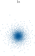
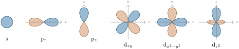
The angular part fixes the shape. An s orbital is spherical; a p orbital has two lobes of opposite signs along its axis, separated by a nodal plane; a d orbital has four lobes of alternating signs (or, for $d_{z^2}$ , two lobes and a ring). The sign of a lobe has no physical meaning by itself — $\psi$ and $-\psi$ describe the same state — but the relative signs of two orbitals decide, in the next chapter, whether they combine into a bond.

Real atomic orbitals, schematic: the lobes show the regions where | | is large, coloured by the sign of (blue positive, orange negative). The d_xz and d_yz orbitals have the shape of d_xy in the planes their names give. — Real atomic orbitals, schematic: the lobes show the regions where $|\psi|$ is large, coloured by the sign of $\psi$ (blue positive, orange negative). The $\mathrm d_{xz}$ and $\mathrm d_{yz}$ orbitals have the shape of $\mathrm d_{xy}$ in the planes their names give.

Method 13.10 (Sketching an orbital from its quantum numbers)

From $l$ , the shape: s (sphere), p (two lobes), d (four lobes, or two lobes and a ring for $d_{z^2}$ ); from the subscript, the orientation.
Count the $l$ angular nodes (planes through the nucleus) and give adjacent lobes opposite signs.
Count the $n - l - 1$ radial nodes: inner shells of opposite sign inside the main lobes (usually left out of sketches).
Scale with $n^2a_0/Z$ : higher $n$ , larger orbital; larger $Z$ , smaller.

13.4 Many-electron atoms

In an atom with several electrons, each electron feels the nucleus screened by the others. The orbitals keep the shapes of the hydrogen ones, with an effective charge $Z^*$ in place of $Z$ , and the energy of a subshell now depends on $l$ as well as on $n$ : an s electron, whose radial distribution has inner maxima close to the nucleus, is screened less than a p electron of the same shell, and a p less than a d.

Definition 13.11 (Slater’s rules)

Slater’s rules estimate the effective nuclear charge $Z^* = Z - \sigma$ felt by an electron. The electrons are grouped as (1s) (2s, 2p) (3s, 3p) (3d) (4s, 4p) (4d) (4f) (5s, 5p) …; the screening constant $\sigma$ of an electron is the sum of the contributions of the other electrons: 0.35 for each other electron of the same group (0.30 within 1s); for an s or p electron, 0.85 for each electron of the shell $n - 1$ and 1.00 for each electron of lower shells; for a d or f electron, 1.00 for every electron of the groups below its own. Groups above contribute nothing.

electron studied	same group	shell $n - 1$	lower shells
1s	0.30	—	—
$n$ s, $n$ p	0.35	0.85	1.00
$n$ d, $n$ f	0.35	1.00	1.00

Slater’s screening constants, per screening electron. The effective principal quantum numbers are

n^* = 1, 2, 3, 3.7, 4.0, 4.2

for

n = 1

to 6.

Method 13.12 (Computing an effective charge)

Write the configuration in Slater’s groups, in order of $n$ , with s and p together and d and f apart.
Pick the electron; add 0.35 for each other electron of its group.
Add 0.85 (s or p electron) or 1.00 (d or f) per electron of the shell just below, and 1.00 per electron deeper.
$Z^* = Z - \sigma$ .

Definition 13.13 (Orbital energy and radius)

In Slater’s model, the orbital energy of an electron of effective charge $Z^*$ and effective principal quantum number $n^*$ is $\varepsilon = -E_RZ^{*2}/n^{*2}$ , and its orbital radius is $n^{*2}a_0/Z^*$ , the most probable radius of a hydrogen-like orbital of charge $Z^*$ .

Proposition 13.14 (Slater energies)

The energy of a group of $k$ electrons of effective charge $Z^*$ is approximately $k\varepsilon = -kE_RZ^{*2}/n^{*2}$ , and the total electronic energy of the atom is the sum over its groups.

Proof. Admitted at this level. ∎

Example 13.15 (Iron: 4s or 3d first?)

Iron is $[\ce{Ar}]\,3\mathrm d^6\,4\mathrm s^2$ . A 4s electron: $\sigma = 0.35 + 14 \times 0.85 + 10 \times 1.00 = 22.25$ , $Z^* = 3.75$ , $\varepsilon = -13.6 \times 3.75^2/3.7^2 = -14.0\,\mathrm{eV}$ . A 3d electron: $\sigma = 5 \times 0.35 + 18 \times 1.00 = 19.75$ , $Z^* = 6.25$ , $\varepsilon = -13.6 \times 6.25^2/9 = -59\,\mathrm{eV}$ . The 3d electrons are much more tightly bound: although 4s is filled first in the building-up order, it is a 4s electron that leaves when iron is ionised, and the iron(II) ion is $[\ce{Ar}]\,3\mathrm d^6$ .

13.5 Using orbital energies and sizes

Proposition 13.16 (Ionisation energy from Slater energies)

In Slater’s model, the first ionisation energy of an atom is the difference between the total energies of the ion and of the atom, computed group by group with the effective charges of each.

Proof. The ionisation energy is $E(\text{ion}) - E(\text{atom})$ ; by Proposition 13.14, both are sums of group energies, and only the group losing the electron changes (inner groups are not screened by outer electrons). ∎

Example 13.17 (Carbon)

Carbon, (2s, 2p) $^4$ : $Z^* = 6 - 2 \times 0.85 - 3 \times 0.35 = 3.25$ ; the group energy is $4 \times (-13.6 \times 3.25^2/4) = -143.6\,\mathrm{eV}$ . The ion $\ce{C+}$ , (2s, 2p) $^3$ : $Z^* = 3.60$ , $3 \times (-13.6 \times 3.60^2/4) = -132.2\,\mathrm{eV}$ . The ionisation energy is $11.5\,\mathrm{eV}$ , against $11.26\,\mathrm{eV}$ measured.

Slater’s effective charge of the valence electron and orbital radius n*2a_0/Z*. Along period 2, Z* grows by 0.65 per element and the atoms shrink; down group 1, Z* stays at 1.30 then 2.20 while n* grows, and the atoms swell. — Slater’s effective charge of the valence electron and orbital radius $n^{*2}a_0/Z^*$ . Along period 2, $Z^*$ grows by 0.65 per element and the atoms shrink; down group 1, $Z^*$ stays at 1.30 then 2.20 while $n^*$ grows, and the atoms swell.

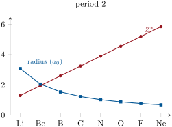
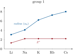
The model reproduces the trends of the Year 1 volume. Along a period, each added proton is screened by only 0.35 of the electron added with it: $Z^*$ rises, the outer orbital contracts and binds more strongly. Down a group, $Z^*$ hardly changes while the outer shell moves out: atoms grow and their ionisation energies fall. Sodium, with $Z^* = 2.20$ for its 3s electron, has an orbital radius of $9/2.2 = 4.1a_0$ ; chlorine, with $Z^* = 6.10$ for a 3p electron, $9/6.1 = 1.5a_0$ .

13.6 Exercises

Exercise 13.1 ★

Give the quantum numbers $n$ and $l$ , the number of radial nodes and of angular nodes of a 3p and of a 4d orbital.

Solution

Solution of Exercise 13.1.

3p: $n = 3$ , $l = 1$ ; one radial node ( $n - l - 1$ ) and one angular node. 4d: $n = 4$ , $l = 2$ ; one radial node and two angular nodes.

Exercise 13.2 ★

Show from $R_{2p}$ that the most probable radius of a 2p electron of hydrogen is $4a_0$ , and give it in picometres.

Solution

Solution of Exercise 13.2.

$P_{2p} \propto r^4\mathrm e^{-r}$ ( $r$ in $a_0$ ): $d\ln P/dr = 4/r - 1 = 0$ for $r = 4$ : $4a_0 = 212\,\mathrm{pm}$ .

Exercise 13.3 ★

Compute the probability of finding the 1s electron of hydrogen closer to the nucleus than $a_0$ .

Solution

Solution of Exercise 13.3.

$1 - \mathrm e^{-2}(1 + 2 + 2) = 1 - 5\mathrm e^{-2} = 0.323$ .

Exercise 13.4 ★

Sketch the $3\mathrm d_{xy}$ orbital: lobes, signs, nodal planes. How many radial nodes does it have?

Solution

Solution of Exercise 13.4.

Four lobes pointing between the $x$ and $y$ axes, in the $xy$ plane, of alternating signs (positive where $xy > 0$ ); the nodal planes are $xz$ and $yz$ . Radial nodes: $n - l - 1 = 0$ .

Exercise 13.5 ★★

Compute Slater’s effective charge for a 2p electron of oxygen and the orbital radius it gives.

Solution

Solution of Exercise 13.5.

Oxygen, $(1\mathrm s)^2(2\mathrm s, 2\mathrm p)^6$ : $\sigma = 5 \times 0.35 + 2 \times 0.85 = 3.45$ , $Z^* = 4.55$ ; radius $4/4.55 = 0.88a_0$ , $47\,\mathrm{pm}$ .

Exercise 13.6 ★★

Using the example of iron, explain why the configuration of $\ce{Fe^3+}$ is $[\ce{Ar}]\,3\mathrm d^5$ and not $[\ce{Ar}]\,3\mathrm d^3 4\mathrm s^2$ .

Solution

Solution of Exercise 13.6.

Ionisation removes the least bound electrons. The 4s electrons ( $-14\,\mathrm{eV}$ ) are far less bound than the 3d ones ( $-59\,\mathrm{eV}$ ): both 4s electrons leave first, then one 3d electron, giving $[\ce{Ar}]\,3\mathrm d^5$ .

Exercise 13.7 ★★

Estimate by Slater’s rules the first ionisation energies of lithium and sodium, and compare with the measured 5.39 and $5.14\,\mathrm{eV}$ . Comment.

Solution

Solution of Exercise 13.7.

Lithium, 2s: $Z^* = 3 - 2 \times 0.85 = 1.30$ , $I = 13.6 \times 1.30^2/4 = 5.75\,\mathrm{eV}$ (measured 5.39, 7 % too high). Sodium, 3s: $Z^* = 11 - 8 \times 0.85 - 2 \times 1.00 = 2.20$ , $I = 13.6 \times 2.20^2/9 = 7.3\,\mathrm{eV}$ (measured 5.14): the rules, a rough model, overestimate the binding of the outer electron, more and more down the group.

Exercise 13.8 ★★

Compute $Z^*$ and the orbital radius of the outer electron of sodium and of chlorine, and explain why the sodium atom is the larger.

Solution

Solution of Exercise 13.8.

Sodium: $Z^* = 2.20$ , radius $9/2.20 = 4.1a_0$ ( $216\,\mathrm{pm}$ ). Chlorine, 3p: $\sigma = 6 \times 0.35 + 8 \times 0.85 + 2 \times 1.00 = 10.90$ , $Z^* = 6.10$ , radius $9/6.10 = 1.5a_0$ ( $78\,\mathrm{pm}$ ). Same shell, but the outer electron of chlorine feels almost three times the charge, and is pulled in.

Exercise 13.9 ★★

Show that the 1s and 2s orbitals of hydrogen are orthogonal, $\int\psi_{1s}\psi_{2s}\,dV = 0$ .

Solution

Solution of Exercise 13.9.

Both have the angular part $1/\sqrt{4\pi}$ , so the integral reduces to

\int_0^\infty R_{1s}R_{2s}r^2\,dr \propto \int_0^\infty (2 - r)r^2\mathrm e^{-3r/2}\,dr = 2 \times \frac{2!}{(3/2)^3} - \frac{3!}{(3/2)^4} = \frac{32}{27} - \frac{32}{27} = 0 .

Exercise 13.10 ★★★

Write $R_{2p} = N\rho\,\mathrm e^{-\rho/2}$ and find the constant $N$ that normalises it ( $Z = 1$ , $r$ in units of $a_0$ ).

Solution

Solution of Exercise 13.10.

$\int_0^\infty N^2r^2\mathrm e^{-r}r^2\,dr = N^2 \times 4! = 1$ : $N = 1/\sqrt{24} = 1/(2\sqrt6)$ , as in the table.

Exercise 13.11 ★★★

Compare the mean radius and the most probable radius of a 1s electron, and explain from the shape of $P(r)$ why they differ.

Solution

Solution of Exercise 13.11.

$\langle r\rangle = 1.5a_0$ , most probable radius $a_0$ . $P(r) = 4r^2\mathrm e^{-2r}$ rises steeply from zero and falls slowly: the long tail at large $r$ weighs more in the mean than in the position of the maximum.

Exercise 13.12 ★★★

Find the nodal surface of the $\mathrm p_z$ orbital and show that $\psi_{2p_z}$ changes sign across it. What is the probability density on that surface?

Solution

Solution of Exercise 13.12.

$Y_{p_z} \propto z/r = \cos\theta$ vanishes for $\theta = \pi/2$ : the $xy$ plane. $\psi$ has the sign of $z$ , positive above, negative below. On the plane the probability density is zero.

13.7 Problem: Where Is the Electron?

Problem 13.1

Weekend problem — the 1s orbital of hydrogen and its radii, the probability of finding the electron beyond a given distance, the nodes and maxima of 2s and 2p, and Slater’s estimate of the ionisation energies of carbon, nitrogen and oxygen

Data: $a_0 = 52.9\,\mathrm{pm}$ ; $E_R = 13.6\,\mathrm{eV}$ ; measured first ionisation energies ( $\mathrm{eV}$ ): C 11.26, N 14.53, O 13.62. $\psi_{1s} = \pi^{-1/2}a_0^{-3/2}\, \mathrm e^{-r/a_0}$ .

Part I — The 1s orbital.

Check that $\psi_{1s}$ is normalised, using $dV = 4\pi r^2\,dr$ .
Write the radial distribution function $P(r)$ .
Find the most probable radius.
Compute the mean radius.
Why is the mean larger than the most probable radius?
The probability density is largest at the nucleus, yet $P(0) = 0$ . Explain.
Give the most probable radius in picometres.

Part II — Beyond a radius.

Show that the probability of finding the electron farther than $r_0 = xa_0$ is $\mathrm e^{-2x}(1 + 2x + 2x^2)$ .
Compute it for $r_0 = a_0$ .
Compute it for $r_0 = 2a_0$ .
Find by trial the radius of the sphere that contains the electron with a probability of 0.90.
In what sense does an atom have no edge, and in what sense a size?

Part III — 2s and 2p.

Give the nodes of 2s and of 2p (number, kind, position).
Where does $R_{2s}$ change sign?
Find the most probable radius of 2p.
Find the two maxima of $P_{2s} \propto r^2(2 - r)^2\mathrm e^{-r}$ ( $r$ in units of $a_0$ ).
Which of 2s and 2p has electron density closer to the nucleus? What does it imply in a many-electron atom?
How do these radii change for the hydrogen-like ion $\ce{C^5+}$ ?

Part IV — Carbon, nitrogen, oxygen.

Compute Slater’s $Z^*$ of a 2p electron in C, N and O.
Compute the corresponding orbital energies.
Estimate the first ionisation energy of carbon as a difference of group energies.
Same for nitrogen.
Same for oxygen, and compare the three with the measured values.
Which feature of the measured values does the model miss, and why?
State the probability of finding the 1s electron of hydrogen farther than $2a_0$ .

Solution

Solution of Problem 13.1.

1. $\int|\psi|^2\,dV = \frac{4\pi}{\pi a_0^3}\int_0^\infty r^2\mathrm e^{-2r/a_0}\,dr = \frac{4}{a_0^3} \times \frac{a_0^3}{4} = 1$ . 2. $P(r) = 4\pi r^2|\psi|^2 = (4/a_0^3)\,r^2\mathrm e^{-2r/a_0}$ . 3. $dP/dr = 0$ : $2/r - 2/a_0 = 0$ , $r = a_0$ . 4. $\langle r\rangle = (4/a_0^3)\int_0^\infty r^3\mathrm e^{-2r/a_0}\,dr = (4/a_0^3) \times 6(a_0/2)^4 = 1.5a_0$ . 5. The distribution is skewed, with a long tail at large $r$ . 6. $|\psi|^2$ is a density per unit volume, largest at the nucleus; $P(r)$ counts the volume of the shell, $4\pi r^2\,dr$ , which vanishes at $r = 0$ . 7. $52.9\,\mathrm{pm}$ . 8. With $x = r/a_0$ : $\int_{x_0}^\infty 4x^2\mathrm e^{-2x}\,dx$ ; by parts twice, $= \mathrm e^{-2x_0}(2x_0^2 + 2x_0 + 1)$ . 9. $5\mathrm e^{-2} = 0.677$ . 10. $13\mathrm e^{-4} = 0.238$ . 11. $\mathrm e^{-2x}(1 + 2x + 2x^2) = 0.10$ for $x \approx 2.66$ : $141\,\mathrm{pm}$ . 12. The density never vanishes at any distance: no edge. But 90 % of the probability lies within $141\,\mathrm{pm}$ : a practical size. 13. 2s: one radial node (sphere of radius $2a_0$ ), no angular node. 2p: one angular node (a plane), no radial node. 14. At $r = 2a_0$ . 15. $4a_0$ (exercise 2). 16. $d\ln P/dr = 2/r - 2/(2 - r) - 1 = 0$ gives $r^2 - 6r + 4 = 0$ , $r = 3 \pm \sqrt5$ : $0.76a_0$ (small inner maximum) and $5.24a_0$ (main maximum). 17. 2s, through its inner maximum. In a many-electron atom a 2s electron penetrates the 1s shell, is less screened than a 2p electron and lies lower in energy. 18. All radii are divided by $Z = 6$ : 2p at $0.67a_0$ ( $35\,\mathrm{pm}$ ); 2s maxima at $0.13a_0$ and $0.87a_0$ . 19. C 3.25, N 3.90, O 4.55. 20. $\varepsilon = -13.6\,Z^{*2}/4$ : C $-35.9\,\mathrm{eV}$ , N $-51.7\,\mathrm{eV}$ , O $-70.4\,\mathrm{eV}$ . 21. As in the chapter: $11.5\,\mathrm{eV}$ (measured 11.26). 22. N: atom $5 \times (-13.6 \times 3.90^2/4) = -258.6\,\mathrm{eV}$ ; $\ce{N+}$ , $Z^* = 4.25$ , $4 \times (-13.6 \times 4.25^2/4) = -245.7\,\mathrm{eV}$ ; $I = 12.9\,\mathrm{eV}$ . 23. O: atom $6 \times (-13.6 \times 4.55^2/4) = -422.3\,\mathrm{eV}$ ; $\ce{O+}$ , $Z^* = 4.90$ , $5 \times (-13.6 \times 4.90^2/4) = -408.2\,\mathrm{eV}$ ; $I = 14.2\,\mathrm{eV}$ . Model 11.5, 12.9, 14.2; measured 11.26, 14.53, 13.62. 24. The measured energy of oxygen is lower than that of nitrogen: in oxygen the fourth 2p electron must share an orbital with another, and their repulsion makes it easier to remove, while nitrogen’s three unpaired p electrons form a stable half-filled subshell. Slater’s rules treat all electrons of a group alike and know nothing of pairing. 25. The 1s electron of hydrogen is farther than $2a_0$ with probability $\boldsymbol{13\mathrm e^{-4} \approx 0.238}$ .

Terms defined in this chapter

See all 852 terms in the glossary