University Chemistry — Year 2 · Bachelor Year 2

3Chemical Potential and Mixtures

In winter a truck spreads salt on an icy road and the ice melts at $-10\,{}^{\circ}\mathrm{C}$ ; the coolant of a car engine, water with a third of ethane-1,2-diol, neither freezes in the night frost nor boils under a hot bonnet. A dissolved substance lowers the freezing point of its solvent and raises its boiling point, and, for dilute solutions, by an amount that depends on the number of dissolved particles and not on what they are. The tool that explains it is the chemical potential, the partial derivative of the Gibbs energy with respect to the amount of one constituent. It tells where each species “wants to go”, between phases and through reactions, and it turns the activities that the Year 1 volume used as recipes into derived quantities.

You already know

Chapter 2: the Gibbs energy $G = H - TS$ , $\dd G = V\dd p - S\dd T + \Delta_r G\,\dd\xi$ , the evolution criterion $\Delta_r G\, \dd\xi \leq 0$ . The Year 1 volume wrote the activity of a gas as $p_i/p^\circ$ , of a solute as $c_i/c^\circ$ , and 1 for a pure solid or a solvent, and noted that in concentrated ionic solutions activities depart from concentrations, “a correction treated in the Year 2 volume”. From physics: the perfect-gas law, and $(\partial G/\partial p)_T = V$ for a pure substance.

A gritting truck spreads salt on a snowy road. The salt dissolves in the thin film of water on the ice, and the solution freezes at a lower temperature than pure water: the ice melts.

3.1 Partial molar quantities

Mix $50\,\mathrm{mL}$ of water and $50\,\mathrm{mL}$ of ethanol: the volume of the mixture is less than $100\,\mathrm{mL}$ . In a mixture, an extensive quantity is not the sum of the contributions of the pure substances; each constituent contributes according to its surroundings.

Definition 3.1 (Partial molar quantity)

Let $X(T, p, n_1, \dots, n_k)$ be an extensive state function of a phase containing the amounts $n_1, \dots, n_k$ . The partial molar quantity of constituent $i$ is

\bar X_i = \left(\frac{\partial X}{\partial n_i}\right)_{T, p, n_{j \ne i}} ,

the change of $X$ per mole of $i$ added to a large amount of the mixture at fixed $T$ , $p$ and other amounts. For $X = V$ it is the partial molar volume $\bar V_i$ .

Theorem 3.2 (Euler’s identity)

At fixed $T$ and $p$ , $X = \sum_i n_i\bar X_i$ .

Proof. $X$ is extensive: multiplying every amount by $\lambda$ multiplies $X$ by $\lambda$ , $X(T, p, \lambda n_1, \dots, \lambda n_k) = \lambda X(T, p, n_1, \dots, n_k)$ . Differentiate with respect to $\lambda$ at $\lambda = 1$ , with the chain rule: $\sum_i n_i\,\partial X/\partial n_i = X$ . ∎

Proposition 3.3 (Gibbs–Duhem relation)

At fixed $T$ and $p$ , $\sum_i n_i\,\dd\bar X_i = 0$ : in a binary mixture, $x_1\dd\bar X_1 + x_2\dd\bar X_2 = 0$ . The partial molar quantities of the constituents cannot vary independently.

Proof. At fixed $T$ , $p$ , $\dd X = \sum_i\bar X_i\dd n_i$ by definition; Euler’s identity, differentiated, gives $\dd X = \sum_i\bar X_i\dd n_i + \sum_i n_i\dd\bar X_i$ . Subtract. ∎

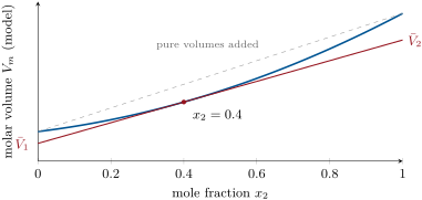
The tangent construction. The molar volume of a model binary mixture (blue) lies below the straight line joining the pure volumes: mixing contracts. The tangent at a composition cuts the two edges at the partial molar volumes V_1 and V_2 of that composition. — The tangent construction. The molar volume of a model binary mixture (blue) lies below the straight line joining the pure volumes: mixing contracts. The tangent at a composition cuts the two edges at the partial molar volumes $\bar V_1$ and $\bar V_2$ of that composition.

Method 3.4 (Partial molar quantities from a curve)

Plot the molar quantity $X_m = X/(n_1 + n_2)$ against $x_2$ . At the composition of interest draw the tangent: it cuts the axis $x_2 = 0$ at $\bar X_1$ and the axis $x_2 = 1$ at $\bar X_2$ . (Proof: $X_m = x_1\bar X_1 + x_2\bar X_2$ and, by Gibbs–Duhem, $\dd X_m/\dd x_2 = \bar X_2 - \bar X_1$ .)

3.2 The chemical potential

Definition 3.5 (Chemical potential)

The chemical potential of constituent $i$ in a phase is its partial molar Gibbs energy,

\mu_i = \left(\frac{\partial G}{\partial n_i}\right)_{T, p, n_{j\ne i}} ,

in $\mathrm{J}/\mathrm{mol}$ . Its value when $i$ is in its standard state is its standard chemical potential $\mu_i^\circ(T)$ , equal to the standard molar Gibbs energy of $i$ .

For a phase whose amounts can change (by reaction, or by exchange with another phase),

\dd G = V\dd p - S\dd T + \sum_i\mu_i\,\dd n_i ,\qquad G = \sum_i n_i\mu_i ,

the second relation by Euler’s identity. With a single reaction, $\dd n_i = \nu_i\dd\xi$ , and comparing with Proposition 2.12:

\Delta_r G = \sum_i\nu_i\mu_i .

The reaction Gibbs energy is the balance of the chemical potentials of the products and of the reactants.

Theorem 3.6 (Equilibrium between phases)

A constituent present in two phases $\alpha$ and $\beta$ of a closed system at uniform $T$ and $p$ is at equilibrium between them if and only if $\mu_i^\alpha = \mu_i^\beta$ . Otherwise it passes spontaneously from the phase where its chemical potential is higher to the phase where it is lower.

Proof. The transfer $i^\alpha \to i^\beta$ is a “reaction” with $\nu^\alpha = -1$ , $\nu^\beta = +1$ , so $\Delta_r G = \mu_i^\beta - \mu_i^\alpha$ . By the evolution criterion it advances ( $\dd\xi > 0$ ) only if $\mu_i^\beta < \mu_i^\alpha$ , recedes if $\mu_i^\beta > \mu_i^\alpha$ , and is at equilibrium if they are equal. ∎

The chemical potential plays for matter the part that temperature plays for heat: heat flows from hot to cold, a species from high to low $\mu$ .

3.3 Ideal systems and activities

Proposition 3.7 (Chemical potential of a perfect gas)

In a mixture of perfect gases, a gas of partial pressure $p_i$ has

\mu_i = \mu_i^\circ(T) + RT\ln\frac{p_i}{p^\circ} .

Proof. For one mole of a pure perfect gas, $(\partial\mu/\partial p)_T = V_m = RT/p$ ; integrating from $p^\circ$ to $p$ gives $\mu = \mu^\circ + RT\ln(p/p^\circ)$ . In a mixture of perfect gases each gas behaves as if alone in the volume, at its partial pressure: replace $p$ by $p_i$ . ∎

Definition 3.8 (Ideal mixture, ideal dilute solution)

A liquid (or solid) mixture is an ideal mixture if, for every constituent and every composition, $\mu_i = \mu_i^*(T, p) + RT\ln x_i$ , where $\mu_i^*$ is the chemical potential of the pure liquid $i$ . A solution is an ideal dilute solution if the solvent obeys this law and each solute obeys $\mu_j = \mu_j^\circ(T) + RT\ln(c_j/c^\circ)$ , with a standard state that is a hypothetical solution at $c^\circ = 1\,\mathrm{mol}/\mathrm{L}$ behaving as if infinitely dilute.

Molecules of similar size and shape whose interactions do not depend on the partner (benzene and toluene, two isotopic forms of a molecule) form nearly ideal mixtures; dilute solutions behave ideally because each solute particle is surrounded by solvent alone.

Theorem 3.9 (Raoult’s law)

Above an ideal liquid mixture, with the vapour a perfect gas, the partial pressure of each constituent is proportional to its mole fraction in the liquid: $p_i = x_i\,p_i^*$ , where $p_i^*$ is the vapour pressure of the pure liquid at the same temperature (Raoult’s law).

Proof. At equilibrium $\mu_i(\text{liquid}) = \mu_i(\text{vapour})$ : $\mu_i^* + RT\ln x_i = \mu_i^\circ + RT\ln(p_i/p^\circ)$ . For the pure liquid ( $x_i = 1$ , $p_i = p_i^*$ ): $\mu_i^* = \mu_i^\circ + RT\ln(p_i^*/p^\circ)$ . Subtracting, $RT\ln x_i = RT\ln(p_i/p_i^*)$ . (The weak dependence of $\mu_i^*$ on the pressure is neglected.) ∎

Proposition 3.10 (Henry’s law)

For a dilute solute $j$ in equilibrium with its vapour, $p_j = k_{H,j}\,x_j$ (or $c_j = H_j\,p_j$ ): the partial pressure of a dilute solute is proportional to its amount in the solution (Henry’s law). The Henry constant $k_{H,j}$ depends on the solute, the solvent and the temperature, and is not the vapour pressure of the pure solute.

Proof. Equate $\mu_j^\circ(\text{solution}) + RT\ln(c_j/c^\circ)$ and $\mu_j^\circ(\text{gas}) + RT\ln(p_j/p^\circ)$ : $c_j/p_j$ is a function of $T$ alone. The constant contains the interactions of $j$ with the solvent, not with itself. ∎

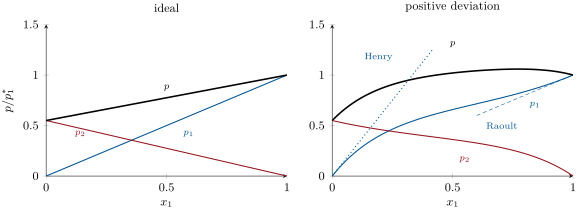
Vapour pressures over a binary liquid at fixed temperature, in units of p_1* (model mixture). Left, an ideal mixture: straight lines (Raoult). Right, a mixture whose unlike molecules attract each other less than like ones: the pressures lie above the ideal lines. Near x_1 = 1, constituent 1 follows Raoult’s line (dashed); near x_1 = 0, it follows a Henry line (dotted) of a different slope. — Vapour pressures over a binary liquid at fixed temperature, in units of $p_1^*$ (model mixture). Left, an ideal mixture: straight lines (Raoult). Right, a mixture whose unlike molecules attract each other less than like ones: the pressures lie above the ideal lines. Near $x_1 = 1$ , constituent 1 follows Raoult’s line (dashed); near $x_1 = 0$ , it follows a Henry line (dotted) of a different slope.

Example 3.11 (Carbon dioxide in a soda)

At $25\,{}^{\circ}\mathrm{C}$ the Henry constant of carbon dioxide in water is $H = 3.4 \times 10^{-4}\,\mathrm{mol}/(\mathrm{m}^{3}\,\mathrm{Pa})$ , that is $0.034\,\mathrm{mol}/(\mathrm{L}\,\mathrm{bar})$ . A bottle sealed under $4\,\mathrm{bar}$ of $\ce{CO2}$ holds $0.034 \times 4 = 0.14\,\mathrm{mol}/\mathrm{L}$ of dissolved gas, about $6\,\mathrm{g}/\mathrm{L}$ . Opened, the gas above it is the air, where $p_{\ce{CO2}} \approx 4 \times 10^{-4}\,\mathrm{bar}$ : the drink is ten thousand times supersaturated and fizzes until it goes flat.

Proposition 3.12 (Activities from chemical potentials)

In every case met so far, $\mu_i = \mu_i^\circ(T) + RT\ln a_i$ , where $a_i$ is the activity of the Year 1 volume: $p_i/p^\circ$ for a perfect gas, $c_i/c^\circ$ for a solute in an ideal dilute solution, $x_i$ (close to 1) for the solvent, and 1 for a pure solid or liquid alone in its phase.

Proof. For the gas and the dilute solute this is the content of Proposition 3.7 and of the definition of the ideal dilute solution. For a constituent of an ideal mixture take its standard state as the pure liquid: $a_i = x_i$ , close to 1 for a solvent. A pure solid or liquid is its own standard state (its weak dependence on the pressure neglected): $\mu = \mu^\circ$ , $a = 1$ . ∎

Proposition 3.13 (Reaction Gibbs energy and quotient)

For a reaction $0 = \sum_i\nu_i\mathrm A_i$ ,

\Delta_r G = \Delta_r G^\circ(T) + RT\ln Q, \qquad Q = \prod_i a_i^{\nu_i} .

Proof. $\Delta_r G = \sum_i\nu_i\mu_i = \sum_i\nu_i\mu_i^\circ + RT\sum_i\nu_i\ln a_i = \Delta_r G^\circ + RT\ln\prod_i a_i^{\nu_i}$ . ∎

This is the bridge between the Gibbs energy of Chapter 2 and the reaction quotient of the Year 1 volume. The next chapter crosses it.

Method 3.14 (Choosing the reference state of an activity)

Gas: the pure perfect gas at $p^\circ$ ; $a = p_i/p^\circ$ .
Solvent, or a constituent of a mixture of comparable amounts: the pure liquid; $a = \gamma_i x_i$ (Raoult reference, $\gamma_i \to 1$ as $x_i \to 1$ ).
Solute: the ideal solution at $c^\circ$ ; $a = \gamma_j c_j/c^\circ$ (Henry reference, $\gamma_j \to 1$ at infinite dilution).
Pure solid, pure liquid alone in its phase: $a = 1$ .

History — François-Marie Raoult

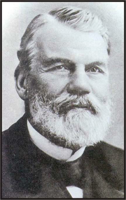
François-Marie Raoult (1830–1901), professor of chemistry at Grenoble, measured during the 1880s the freezing points and then the vapour pressures of hundreds of solutions, and found that, for dilute solutions, the lowering depends on the number of dissolved molecules and not on their nature. His measurements became a way of weighing molecules, and supported the young theory of ions in solution. (Photograph: public domain, Wikimedia Commons.)

3.4 Real mixtures

Definition 3.15 (Activity coefficient)

In a real mixture the chemical potential is written $\mu_i = \mu_i^\circ + RT\ln a_i$ with $a_i = \gamma_i x_i$ (Raoult reference) or $a_i = \gamma_i c_i/c^\circ$ (Henry reference). The factor $\gamma_i$ is the activity coefficient: it measures the departure from the ideal law, and tends to 1 in the limit where the reference law holds.

A coefficient above 1 means that the molecule is less stabilised by its neighbours in the mixture than in the reference state (positive deviation, as in the figure above); below 1, more stabilised. By Gibbs–Duhem, the coefficients of the two constituents of a binary mixture are linked: in the one-parameter model used for the figure, $\ln\gamma_1 = Ax_2^2$ and $\ln\gamma_2 = Ax_1^2$ , and $x_1\,\dd\ln\gamma_1 + x_2\,\dd\ln\gamma_2 = 0$ holds identically.

For ions, which interact at long range, departures appear at small concentrations.

Definition 3.16 (Ionic strength)

The ionic strength of a solution is $I = \frac12\sum_i z_i^2\,b_i$ , where $b_i$ is the molality of ion $i$ (amount per kilogram of solvent) and $z_i$ its charge number.

Proposition 3.17 (Debye–Hückel limiting law)

In a very dilute electrolyte solution, the mean activity coefficient of the ions of a salt obeys $\log\gamma_\pm = -A\,|z_+z_-|\sqrt{I/b^\circ}$ , with $A \approx 0.51$ for water at $25\,{}^{\circ}\mathrm{C}$ and $b^\circ = 1\,\mathrm{mol}/\mathrm{kg}$ .

Proof. Admitted at this level. ∎

Remark 3.18 (Range and origin)

The law comes from a model in which each ion is surrounded by a diffuse “atmosphere” of opposite charge, which lowers its chemical potential; the model is beyond this course, but its constant $A$ follows from the permittivity and density of water and the temperature. It is accurate below about $I = 0.01\,\mathrm{mol}/\mathrm{kg}$ . The same ionic atmosphere slows the ions in an electric field, and explains why the molar conductivity of a strong electrolyte falls as $\Lambda = \Lambda^\circ - K\sqrt c$ (Kohlrausch’s square-root law) rather than staying at its limiting value: the limit of Kohlrausch’s law met in the Year 1 volume.

Example 3.19 (A centimolar salt)

For sodium chloride at $b = 0.010\,\mathrm{mol}/\mathrm{kg}$ , $I = \frac12(0.010 + 0.010) = 0.010\,\mathrm{mol}/\mathrm{kg}$ and $\log\gamma_\pm = -0.51 \times 0.10$ : $\gamma_\pm = 0.89$ . Already at one hundredth of a mole per kilogram, taking the concentration for the activity is an error of 11 %; for a 2:2 salt such as magnesium sulfate at the same molality, $I = 0.040$ and $\gamma_\pm = 0.62$ .

3.5 Colligative properties

Definition 3.20 (Colligative property)

A colligative property of a dilute solution is one that depends on the amount of dissolved particles per amount of solvent and not on their nature: the lowering of the vapour pressure, of the freezing point, the raising of the boiling point, and the osmotic pressure. The constants of the freezing-point and boiling-point laws below are the cryoscopic constant $K_f$ and the ebullioscopic constant $K_b$ of the solvent.

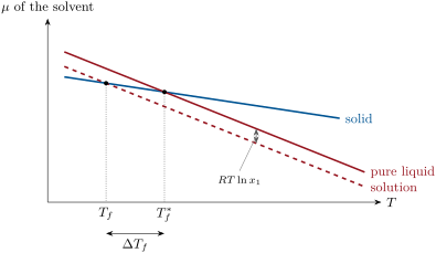
Chemical potential of the solvent against temperature (schematic, at fixed pressure). The stable phase is the one of lowest . Dissolving a solute lowers the liquid’s line by RT x_1 < 0; it now meets the solid’s line at a lower temperature: the solution freezes below the pure solvent. — Chemical potential of the solvent against temperature (schematic, at fixed pressure). The stable phase is the one of lowest $\mu$ . Dissolving a solute lowers the liquid’s line by $RT\ln x_1 < 0$ ; it now meets the solid’s line at a lower temperature: the solution freezes below the pure solvent.

Theorem 3.21 (Freezing-point depression)

A dilute solution of a solute that does not enter the solid begins to freeze at $T_f = T_f^* - \Delta T_f$ , with

\Delta T_f = K_f\,b, \qquad K_f = \frac{R\,T_f^{*2}\,M_1}{\Delta_{\text{fus}}H_1} ,

$b$ being the total molality of the dissolved particles and $M_1$ the molar mass of the solvent (in $\mathrm{kg}/\mathrm{mol}$ ). For finite concentrations the exact relation for an ideal solution is $\ln x_1 = -\frac{\Delta_{\text{fus}}H_1}{R} \left(\frac{1}{T_f} - \frac{1}{T_f^*}\right)$ .

Proof. At the freezing point, pure solid solvent and solvent in the solution are in equilibrium: $\mu_1^{\text{s}}(T) = \mu_1^{*\text{l}}(T) + RT\ln x_1$ , so $\ln x_1 = -\Delta_{\text{fus}}G_1(T)/(RT)$ , with $\Delta_{\text{fus}}G_1 = \mu_1^{*\text{l}} - \mu_1^{\text{s}}$ , zero at $T_f^*$ . By Gibbs–Helmholtz, $\dd(\Delta_{\text{fus}}G_1/T)/\dd T = -\Delta_{\text{fus}}H_1/T^2$ ; integrating from $T_f^*$ to $T_f$ with $\Delta_{\text{fus}}H_1$ constant gives the exact relation. For a dilute solution, $\ln x_1 = \ln(1 - x_2) \approx -x_2$ and $\frac1{T_f} - \frac1{T_f^*} \approx -\Delta T_f/T_f^{*2}$ , so $x_2 = \Delta_{\text{fus}}H_1\Delta T_f/(RT_f^{*2})$ ; finally $x_2 \approx n_2/n_1 = b\,M_1$ . ∎

Proposition 3.22 (Boiling-point elevation)

A dilute solution of a non-volatile solute boils at $T_b^* + \Delta T_b$ with $\Delta T_b = K_b\,b$ , $K_b = RT_b^{*2}M_1/\Delta_{\text{vap}}H_1$ .

Proof. The same, with the vapour in place of the solid: $\mu_1^{*\text{l}} + RT\ln x_1 = \mu_1^{\text{v}}$ ; the solvent’s line is lowered, and now meets the vapour’s line at a higher temperature. ∎

Example 3.23 (Water)

With $\Delta_{\text{fus}}H = 333.4\,\mathrm{J}/\mathrm{g} = 6.007\,\mathrm{kJ}/\mathrm{mol}$ at $273.15\,\mathrm{K}$ : $K_f = 8.314 \times 273.15^2 \times 0.018015/6007 = 1.86\,\mathrm{K}\,\mathrm{kg}/\mathrm{mol}$ . With $\Delta_{\text{vap}}H = 40.65\,\mathrm{kJ}/\mathrm{mol}$ at $373.12\,\mathrm{K}$ : $K_b = 0.513\,\mathrm{K}\,\mathrm{kg}/\mathrm{mol}$ . Sea water, $35\,\mathrm{g}$ of salt per kilogram, counted as sodium chloride (two particles per formula): $b = 2 \times 35/58.44/0.965 = 1.24\,\mathrm{mol}/\mathrm{kg}$ , so the dilute law predicts $-2.3\,{}^{\circ}\mathrm{C}$ , an overestimate: at this concentration the ions are far from ideal, and sea salt is not all sodium chloride.

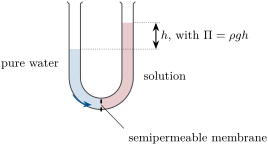
Definition 3.24 (Semipermeable membrane, osmotic pressure)

A semipermeable membrane lets the solvent through and not the solute. When it separates a solution from the pure solvent, the solvent flows into the solution; the osmotic pressure $\Pi$ is the excess pressure that must be applied to the solution to stop that flow.

Theorem 3.25 (van ’t Hoff’s osmotic law)

For a dilute solution, $\Pi = c\,RT$ , where $c$ is the total concentration of solute particles.

Proof. At equilibrium the solvent has the same chemical potential on both sides: $\mu_1^*(T, p) = \mu_1^*(T, p + \Pi) + RT\ln x_1$ . Since $(\partial\mu_1^*/ \partial p)_T = V_{m,1}$ , nearly constant for a liquid, $\mu_1^*(T, p + \Pi) - \mu_1^*(T, p) = \Pi V_{m,1}$ , so $\Pi V_{m,1} = -RT\ln x_1 \approx RT x_2 \approx RT\,n_2/n_1$ . With $n_1V_{m,1} \approx V$ (dilute), $\Pi = n_2RT/V$ . ∎

Osmosis in a U-tube. Water passes through the membrane into the solution until the extra hydrostatic pressure of the higher column equals the osmotic pressure; then the chemical potentials of water on the two sides are equal.

Method 3.26 (Molar mass by a colligative property)

Dissolve a known mass $m_2$ of the substance in a known mass $m_1$ of solvent (or a known volume $V$ of solution).
Measure $\Delta T_f$ (or $\Delta T_b$ , or $\Pi$ ).
Deduce the molality $b = \Delta T_f/K_f$ (or $c = \Pi/RT$ ), then $n_2 = b\,m_1$ (or $cV$ ) and $M_2 = m_2/n_2$ ; divide by the number of particles per formula if the substance dissociates.

Osmometry suits large molecules (proteins, polymers): a few grams per litre of a protein of $60\,\mathrm{kg}/\mathrm{mol}$ give a few hundred pascals, millimetres of water, but a freezing-point change of only a few thousandths of a kelvin.

3.6 Exercises

Exercise 3.1 ★

Use the tangent construction on the figure of the molar volume (model mixture) at $x_2 = 0.4$ to read $\bar V_1$ and $\bar V_2$ , and check that $x_1\bar V_1 + x_2\bar V_2$ is the molar volume of the mixture.

Solution

Solution of Exercise 3.1.

The tangent at $x_2 = 0.4$ cuts the edges at $\bar V_1 \approx 14$ and $\bar V_2 \approx 49$ (model units). Then $0.6 \times 14 + 0.4 \times 49 = 28.0$ , the molar volume read on the curve at $x_2 = 0.4$ , below the $0.6 \times 18 + 0.4 \times 58 = 34.0$ of the pure volumes.

Exercise 3.2 ★

At $25\,{}^{\circ}\mathrm{C}$ the vapour pressure of water is $3.17\,\mathrm{kPa}$ . Compute, by Raoult’s law, the vapour pressure above a solution of $1.00\,\mathrm{mol}$ of sucrose (non-volatile) in $1.00\,\mathrm{kg}$ of water.

Solution

Solution of Exercise 3.2.

$n(\text{water}) = 1000/18.015 = 55.5\,\mathrm{mol}$ , $x_1 = 55.5/56.5 = 0.982$ ; $p = 0.982 \times 3.17 = 3.11\,\mathrm{kPa}$ : a lowering of 1.8 %.

Exercise 3.3 ★

Compute the concentration of dioxygen dissolved in water in equilibrium with air at $1.013\,\mathrm{bar}$ and $25\,{}^{\circ}\mathrm{C}$ ( $H(\ce{O2}) = 1.3 \times 10^{-5}\,\mathrm{mol}/(\mathrm{m}^{3}\,\mathrm{Pa})$ , $20.95\,\%$ of dioxygen), in $\mathrm{mol}/\mathrm{L}$ and $\mathrm{mg}/\mathrm{L}$ .

Solution

Solution of Exercise 3.3.

$p(\ce{O2}) = 0.2095 \times 1.013 \times 10^{5}\,\mathrm{Pa} = 2.12 \times 10^{4}\,\mathrm{Pa}$ ; $c = 1.3 \times 10^{-5} \times 2.12 \times 10^4 = 0.28\,\mathrm{mol}/\mathrm{m}^{3} = 2.8 \times 10^{-4}\,\mathrm{mol}/\mathrm{L}$ , that is $2.8 \times 10^{-4} \times 32.0 \times 10^3 = 8.8\,\mathrm{mg}/\mathrm{L}$ .

Exercise 3.4 ★

For $\ce{N2(g) + 3H2(g) <=> 2NH3(g)}$ at $298\,\mathrm{K}$ , $\Delta_r G^\circ = -32.8\,\mathrm{kJ}/\mathrm{mol}$ . Compute $\Delta_r G$ in a mixture where $p(\ce{N2}) = 1.0\,\mathrm{bar}$ , $p(\ce{H2}) = 0.010\,\mathrm{bar}$ and $p(\ce{NH3}) = 1.0\,\mathrm{bar}$ , and say which way the reaction goes.

Solution

Solution of Exercise 3.4.

$Q = (1.0)^2/[(1.0)(0.010)^3] = 1.0 \times 10^6$ ; $RT\ln Q = 2.479 \times 13.82 = 34.2\,\mathrm{kJ}/\mathrm{mol}$ ; $\Delta_r G = -32.8 + 34.2 = +1.4\,\mathrm{kJ}/\mathrm{mol} > 0$ : in this mixture, so poor in hydrogen, ammonia decomposes.

Exercise 3.5 ★★

In a binary mixture, the partial molar volume of constituent 1 changes by $\dd\bar V_1 = -0.30\,\mathrm{mL}/\mathrm{mol}$ when $x_2$ goes from 0.30 to 0.31. Using Gibbs–Duhem, find $\dd\bar V_2$ .

Solution

Solution of Exercise 3.5.

Gibbs–Duhem: $x_1\dd\bar V_1 + x_2\dd\bar V_2 = 0$ , so $\dd\bar V_2 = -(0.70/0.30) \times (-0.30) = +0.70\,\mathrm{mL}/\mathrm{mol}$ .

Exercise 3.6 ★★

Physiological saline contains $9.0\,\mathrm{g}$ of sodium chloride per litre. Compute its osmotic pressure at $37\,{}^{\circ}\mathrm{C}$ , taking the salt as fully dissociated, and explain why red blood cells keep their shape in it but swell and burst in pure water.

Solution

Solution of Exercise 3.6.

$c(\text{particles}) = 2 \times 9.0/58.44 = 0.308\,\mathrm{mol}/\mathrm{L} = 308\,\mathrm{mol}/\mathrm{m}^{3}$ ; $\Pi = 308 \times 8.314 \times 310 = 7.9 \times 10^{5}\,\mathrm{Pa}$ , about $7.9\,\mathrm{bar}$ . The inside of a red cell has the same osmotic pressure: no net flow of water. In pure water, water enters the cell, which swells and bursts.

Exercise 3.7 ★★

A solution of $2.00\,\mathrm{g}$ of a protein in $100.0\,\mathrm{mL}$ of water has an osmotic pressure of $0.825\,\mathrm{kPa}$ at $25\,{}^{\circ}\mathrm{C}$ . Compute the molar mass of the protein, and the freezing-point depression of this solution.

Solution

Solution of Exercise 3.7.

$c = \Pi/RT = 825/(8.314 \times 298.15) = 0.333\,\mathrm{mol}/\mathrm{m}^{3}$ ; in $1.000 \times 10^{-4}\,\mathrm{m}^{3}$ , $n = 3.33 \times 10^{-5}\,\mathrm{mol}$ , $M = 2.00/3.33 \times 10^{-5} = 6.0 \times 10^{4}\,\mathrm{g}/\mathrm{mol}$ ( $60\,\mathrm{kg}/\mathrm{mol}$ ). $\Delta T_f = 1.86 \times 3.33 \times 10^{-5}/0.100 = 6.2 \times 10^{-4}\,\mathrm{K}$ : unmeasurable, while the osmotic pressure is a column of $8\,\mathrm{cm}$ of water.

Exercise 3.8 ★★

Compute the ionic strength and the mean activity coefficients (limiting law) of: (a) $1.0 \times 10^{-3}\,\mathrm{mol}/\mathrm{kg}$ sodium chloride; (b) $1.0 \times 10^{-3}\,\mathrm{mol}/\mathrm{kg}$ calcium chloride; (c) $1.0 \times 10^{-3}\,\mathrm{mol}/\mathrm{kg}$ magnesium sulfate.

Solution

Solution of Exercise 3.8.

(a) $I = 1.0 \times 10^{-3}\,\mathrm{mol}/\mathrm{kg}$ , $\log\gamma_\pm = -0.51 \times 0.0316$ , $\gamma_\pm = 0.964$ . (b) $I = \frac12(4 \times 1.0 + 1 \times 2.0) \times 10^{-3} = 3.0 \times 10^{-3}\,\mathrm{mol}/\mathrm{kg}$ , $\log\gamma_\pm = -0.51 \times 2 \times 0.0548$ , $\gamma_\pm = 0.879$ . (c) $I = \frac12(4 + 4) \times 10^{-3} = 4.0 \times 10^{-3}\,\mathrm{mol}/\mathrm{kg}$ , $\log\gamma_\pm = -0.51 \times 4 \times 0.0632$ , $\gamma_\pm = 0.74$ .

Exercise 3.9 ★★

A solution of $1.50\,\mathrm{g}$ of an unknown non-volatile, non-dissociating compound in $50.0\,\mathrm{g}$ of water freezes at $-0.310\,{}^{\circ}\mathrm{C}$ . Compute its molar mass.

Solution

Solution of Exercise 3.9.

$b = 0.310/1.86 = 0.167\,\mathrm{mol}/\mathrm{kg}$ ; $n = 0.167 \times 0.0500 = 8.33 \times 10^{-3}\,\mathrm{mol}$ ; $M = 1.50/8.33 \times 10^{-3} = 180\,\mathrm{g}/\mathrm{mol}$ (a hexose sugar, for instance).

Exercise 3.10 ★★★

Show that in the one-parameter model $\ln\gamma_1 = Ax_2^2$ , $\ln\gamma_2 = Ax_1^2$ , the Gibbs–Duhem relation holds, and that the Henry constant of constituent 1 is $k_{H,1} = p_1^*\mathrm e^A$ . For $A = 1.1$ , by what factor does Henry’s slope exceed Raoult’s?

Solution

Solution of Exercise 3.10.

$x_1\,\dd(Ax_2^2) + x_2\,\dd(Ax_1^2) = 2Ax_1x_2(\dd x_2 + \dd x_1) = 0$ since $x_1 + x_2 = 1$ . As $x_1 \to 0$ , $\gamma_1 \to \mathrm e^{A}$ and $p_1 = \gamma_1x_1p_1^* \approx \mathrm e^{A}p_1^*\,x_1$ : $k_{H,1} = p_1^*\mathrm e^A$ . For $A = 1.1$ , $\mathrm e^{1.1} = 3.0$ : Henry’s slope is three times Raoult’s.

Exercise 3.11 ★★★

Explain why a colligative law needs (a) a non-volatile solute for the boiling-point elevation, and (b) a solute that does not enter the solid for the freezing-point depression. What happens to the freezing point of a solvent whose solute forms an ideal solid solution with it in the same proportion as in the liquid?

Solution

Solution of Exercise 3.11.

(a) A volatile solute contributes its own vapour pressure; the vapour is no longer pure solvent and the derivation (pure vapour of the solvent in equilibrium with the solution) fails. (b) If the solute enters the solid, the solid’s chemical potential is lowered too, by $RT\ln x_1^{\text{s}}$ . If the solid solution has the same composition as the liquid, both lines move down by the same amount and the freezing point does not change: the depression needs a solute rejected by the crystal.

Exercise 3.12 ★★★

A thermometer reads to $0.01\,\mathrm{K}$ . Compute the smallest molality of a non-dissociating solute detectable in water by cryoscopy and by ebullioscopy, and the corresponding osmotic pressure at $25\,{}^{\circ}\mathrm{C}$ . Which method is the most sensitive, and why are osmometers used for polymers?

Solution

Solution of Exercise 3.12.

Cryoscopy: $b_{\min} = 0.01/1.86 = 5.4 \times 10^{-3}\,\mathrm{mol}/\mathrm{kg}$ ; ebullioscopy: $0.01/0.513 = 1.9 \times 10^{-2}\,\mathrm{mol}/\mathrm{kg}$ . At $5.4 \times 10^{-3}\,\mathrm{mol}/\mathrm{L} = 5.4\,\mathrm{mol}/\mathrm{m}^{3}$ , $\Pi = 5.4 \times 8.314 \times 298 = 1.3 \times 10^{4}\,\mathrm{Pa}$ , more than a metre of water; an osmometer reads a few pascals. Osmometry is by far the most sensitive, which is why it measures the large molar masses of polymers, whose molalities are tiny.

3.7 Problem: The Radiator in Winter

Problem 3.1

Weekend problem — an ideal mixture of water and ethane-1,2-diol, the cryoscopic law and its constant, the freezing of a coolant, and how much diol keeps an engine liquid at $-20\,{}^{\circ}\mathrm{C}$

The coolant of an engine is a mixture of water and ethane-1,2-diol ( $\ce{HOCH2CH2OH}$ , $M = 62.07\,\mathrm{g}/\mathrm{mol}$ , boiling point $197\,{}^{\circ}\mathrm{C}$ , non-volatile here). Water: $M = 18.015\,\mathrm{g}/\mathrm{mol}$ , freezing point $273.15\,\mathrm{K}$ , enthalpy of fusion $333.4\,\mathrm{J}/\mathrm{g}$ , boiling point $373.12\,\mathrm{K}$ under $1.013\,\mathrm{bar}$ , enthalpy of vaporisation $40.65\,\mathrm{kJ}/\mathrm{mol}$ , vapour pressure $3.17\,\mathrm{kPa}$ at $25\,{}^{\circ}\mathrm{C}$ . The mixture is taken as ideal.

Part I — The mixture.

Write the chemical potential of water in an ideal mixture.
A coolant contains $30\,\%$ of diol by mass. Compute the amounts of diol and water in $100\,\mathrm{g}$ , and the mole fraction of water.
Compute the vapour pressure of water above this coolant at $25\,{}^{\circ}\mathrm{C}$ .
Compute the molality of the diol.
Why is the diol’s own vapour pressure neglected?

Part II — The cryoscopic law.

Write the equality of chemical potentials at the freezing point of the coolant, the solid being pure ice.
Using the Gibbs–Helmholtz relation, derive $\ln x_1 = -\frac{\Delta_{\text{fus}}H}{R}\left(\frac1{T_f} - \frac1{T_f^*}\right)$ .
Linearise it for a dilute solution and obtain $\Delta T_f = K_f b$ .
Compute the molar enthalpy of fusion of water and $K_f$ .
What assumption about the enthalpy of fusion did the integration make?

Part III — Freezing.

Compute the freezing point of the $30\,\%$ coolant with the dilute law.
Compute it with the exact ideal relation.
Which result do you trust more, and why are both only estimates for a real coolant?
At the freezing point, what crystallises?
Cooled further, the remaining liquid becomes richer in diol. Explain why ice keeps forming at lower and lower temperatures.

Part IV — Boiling, and the winter target.

Compute $K_b$ of water.
Compute the boiling-point elevation of the $30\,\%$ coolant at $1.013\,\mathrm{bar}$ .
The radiator is pressurised to $2.0\,\mathrm{bar}$ . Using the Clausius–Clapeyron relation of physics with the enthalpy of vaporisation above, estimate the boiling point of pure water at $2.0\,\mathrm{bar}$ .
Which matters more for the summer, the cap or the diol?
For a coolant liquid down to $-20\,{}^{\circ}\mathrm{C}$ , compute the mole fraction of water required by the exact ideal relation.
Convert it into a mass fraction of diol.
Compute the mass fraction that the dilute law would have given, and explain the difference.
State the mass fraction of diol that keeps the coolant liquid down to $-20\,{}^{\circ}\mathrm{C}$ in the ideal-mixture model.

Solution

Solution of Problem 3.1.

1. $\mu_1 = \mu_1^*(T, p) + RT\ln x_1$ . 2. Diol $30/62.07 = 0.483\,\mathrm{mol}$ , water $70/18.015 = 3.886\,\mathrm{mol}$ ; $x_1 = 3.886/4.369 = 0.889$ . 3. $p = 0.889 \times 3.17 = 2.82\,\mathrm{kPa}$ . 4. $b = 0.483/0.070 = 6.90\,\mathrm{mol}/\mathrm{kg}$ . 5. The diol boils at $197\,{}^{\circ}\mathrm{C}$ : its vapour pressure at room temperature is far below that of water. 6. $\mu_1^{\text{s}}(T_f) = \mu_1^{*\text{l}}(T_f) + RT_f\ln x_1$ . 7. $\ln x_1 = -\Delta_{\text{fus}}G(T)/(RT)$ with $\Delta_{\text{fus}}G = \mu_1^{*\text{l}} - \mu_1^{\text{s}}$ , zero at $T_f^*$ ; Gibbs–Helmholtz, $\dd(\Delta_{\text{fus}}G/T)/\dd T = -\Delta_{\text{fus}}H/T^2$ , integrated from $T_f^*$ to $T_f$ , gives $\Delta_{\text{fus}}G(T_f)/T_f = \Delta_{\text{fus}}H(1/T_f - 1/T_f^*)$ , whence the relation. 8. $\ln x_1 \approx -x_2 \approx -bM_1$ and $1/T_f - 1/T_f^* \approx -\Delta T_f/T_f^{*2}$ : $\Delta T_f = (RT_f^{*2}M_1/\Delta_{\text{fus}}H)\,b$ . 9. $333.4 \times 18.015 = 6007\,\mathrm{J}/\mathrm{mol}$ ; $K_f = 8.314 \times 273.15^2 \times 0.018015/6007 = 1.86\,\mathrm{K}\,\mathrm{kg}/\mathrm{mol}$ . 10. That $\Delta_{\text{fus}}H$ does not change between $T_f$ and $T_f^*$ (it does, by Kirchhoff, about 2 % per $3\,\mathrm{K}$ here). 11. $\Delta T_f = 1.86 \times 6.90 = 12.8\,\mathrm{K}$ : $-12.8\,{}^{\circ}\mathrm{C}$ . 12. $1/T_f = 1/273.15 - (8.314/6007)\ln 0.889$ : $T_f = 261.6\,\mathrm{K}$ , $-11.6\,{}^{\circ}\mathrm{C}$ . 13. The exact ideal relation, which does not assume a dilute solution (here 11 % of the molecules are diol). Both assume an ideal mixture and a constant enthalpy of fusion; water and diol, linked by hydrogen bonds, are not ideal, so the real freezing point differs. 14. Pure ice: the diol stays in the liquid. 15. Removing water as ice lowers $x_1$ in the liquid, and by the relation the equilibrium temperature falls: the coolant freezes over a range of temperatures, not at one point. 16. $K_b = 8.314 \times 373.12^2 \times 0.018015/40\,650 = 0.513\,\mathrm{K}\,\mathrm{kg}/\mathrm{mol}$ . 17. $\Delta T_b = 0.513 \times 6.90 = 3.5\,\mathrm{K}$ . 18. $1/T = 1/373.12 - (8.314/40\,650)\ln(2.0/1.013)$ : $T = 393.5\,\mathrm{K}$ , about $120\,{}^{\circ}\mathrm{C}$ . 19. The cap: $20\,\mathrm{K}$ against $3.5\,\mathrm{K}$ for the diol. 20. $x_1 = \exp[-(6007/8.314)(1/253.15 - 1/273.15)] = 0.811$ . 21. $x_2 = 0.189$ : $w = 0.189 \times 62.07/(0.189 \times 62.07 + 0.811 \times 18.015) = 0.44$ . 22. Dilute law: $b = 20/1.86 = 10.75\,\mathrm{mol}/\mathrm{kg}$ , $w = 10.75 \times 62.07/(1000 + 10.75 \times 62.07) = 0.40$ . The linearisations ( $\ln x_1 \approx -x_2$ , $x_2 \approx bM_1$ ) overstate the lowering per mole of diol at such a high concentration, so the dilute law asks for less diol. 23. In the ideal-mixture model, a coolant with a mass fraction of diol $\boldsymbol{w \approx 0.44}$ stays liquid down to $-20\,{}^{\circ}\mathrm{C}$ .

Terms defined in this chapter

See all 852 terms in the glossary