University Chemistry — Year 2 · Bachelor Year 2

34Statistics of Chemical Measurement

Two laboratories measure the lead in the same tap water and report 9.6 and $11.2\,\text{µ}\mathrm{g}/\mathrm{L}$ . The guideline value for drinking water is $10\,\text{µ}\mathrm{g}/\mathrm{L}$ . Is the water fit to drink? Do the two laboratories even disagree, or are both results the same value seen through the scatter of two measurements? A number from an analysis means nothing without its uncertainty, and this chapter gives the tools to compute it: the statistics of repeated measurements, the propagation of uncertainties through a calculation, calibration by least squares, and the limits below which a method sees nothing.

A water-testing laboratory: sample bottles, a technician pipetting, an elemental analyser behind (illustration).

You already know

The Year 1 volume: measurement uncertainty, standard uncertainty, type A and type B evaluations, expanded uncertainty, relative uncertainty, the normalised deviation $z$ between two values, and the promise of a proof of $u(\bar x) = s/\sqrt n$ and of a general propagation rule. The school volume: the calibration line. Chapter 32: atomic absorption.

34.1 Repeated measurements

Repeat a measurement and the results scatter. We treat each result $x_i$ as a random variable with mean $\mu$ (the value the method would give on average) and standard deviation $\sigma$ ; when many small independent causes add up, the results follow the normal (Gaussian) law, about 68 % of them within $\mu \pm \sigma$ and 95 % within $\mu \pm 1.96\sigma$ .

Definition 34.1 (Dispersion)

For $n$ results $x_1, \dots, x_n$ of mean $\bar x$ , the experimental standard deviation is $s = \sqrt{\sum (x_i - \bar x)^2/(n-1)}$ ; it estimates $\sigma$ . The standard deviation of the mean is the standard deviation of $\bar x$ over many series of $n$ results, estimated by $s/\sqrt n$ .

The divisor $n - 1$ rather than $n$ corrects for the fact that the deviations are taken from $\bar x$ , itself computed from the same data, which makes them slightly too small: $n - 1$ is the number of independent deviations, the degrees of freedom.

Theorem 34.2 (Variance of the mean)

If $x_1, \dots, x_n$ are independent, each of variance $\sigma^2$ , then $\operatorname{var}(\bar x) = \sigma^2/n$ : the standard deviation of the mean is $\sigma/\sqrt n$ .

Proof. For independent variables the variance of a sum is the sum of the variances, and $\operatorname{var}(cX) = c^2\operatorname{var}(X)$ . So $\operatorname{var}(\bar x) = \operatorname{var}\bigl(\tfrac1n\sum x_i\bigr) = \tfrac{1}{n^2}\sum\operatorname{var}(x_i) = \tfrac{1}{n^2}\,n\sigma^2 = \sigma^2/n$ . Replacing $\sigma$ by its estimate $s$ gives the type A standard uncertainty $u(\bar x) = s/\sqrt n$ admitted in the Year 1 volume. ∎

34.2 Confidence intervals

Definition 34.3 (Confidence interval)

A confidence interval at confidence level $1 - \alpha$ (often 95 %) is an interval computed from the data by a rule that, applied to many series, contains the true value in a fraction $1 - \alpha$ of them. For the mean of $n$ results it is $\bar x \pm t\,s/\sqrt n$ , where $t$ is Student’s coefficient for $n - 1$ degrees of freedom and that level.

Proposition 34.4 (Student’s law)

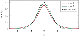
For $n$ independent normal results, $T = (\bar x - \mu)/(s/\sqrt n)$ follows Student’s law with $n - 1$ degrees of freedom, whose density is proportional to $(1 + t^2/\nu)^{-(\nu+1)/2}$ with $\nu = n - 1$ . It is wider than the normal law and tends to it as $n$ grows.

Proof. Admitted at this level. ∎

Dividing by $s$ instead of the unknown $\sigma$ adds the scatter of $s$ itself, which is large when $n$ is small; hence the heavier tails, and coefficients larger than 1.96. The table gives the 95 % coefficients, computed from the density.

Student densities for 2 and 5 degrees of freedom against the normal law, and the two-sided 95 % coefficients, computed by integrating the density (the last line is the normal law).

$\nu = n - 1$	$t$ (95 %)
1	12.706
2	4.303
3	3.182
4	2.776
5	2.571
9	2.262
20	2.086
$\infty$	1.960

Method 34.5 (A confidence interval for a mean)

Compute $\bar x$ and $s$ of the $n$ results; check that no result is grossly out of line.
Read $t$ for $\nu = n - 1$ at the chosen level.
Report $\bar x \pm t\,s/\sqrt n$ , with the uncertainty rounded to one or two significant digits and the mean to the same decimal place.
To compare with a reference value $x_{\mathrm{ref}}$ , compute $|\bar x - x_{\mathrm{ref}}|/(s/\sqrt n)$ : above $t$ , the difference is significant at that level; below, the data do not show a difference (which does not prove there is none).

34.3 Propagation of uncertainty

Theorem 34.6 (Law of propagation of uncertainty)

If $y = f(x_1, \dots, x_n)$ , where the $x_i$ are independent with standard uncertainties $u(x_i)$ small enough for $f$ to be nearly linear over them, then

u^2(y) = \sum_{i=1}^{n}\left(\frac{\partial f}{\partial x_i}\right)^2 u^2(x_i).

Proof. To first order (Taylor), $y - f(\mu_1, \dots, \mu_n) \approx \sum c_i(x_i - \mu_i)$ with $c_i = \partial f/\partial x_i$ at the means. The variance of a linear combination of independent variables is $\sum c_i^2\operatorname{var}(x_i)$ (as in Theorem 34.2); with $\operatorname{var}(x_i) = u^2(x_i)$ this is the result. ∎

Corollary 34.7 (Sums and products)

For a sum or difference, the standard uncertainties add in quadrature: $u^2(x_1 \pm x_2) = u^2(x_1) + u^2(x_2)$ . For a product or quotient $y = x_1^{a}x_2^{b}\cdots$ , the relative uncertainties add in quadrature, each weighted by its exponent: $\bigl(u(y)/y\bigr)^2 = a^2\bigl(u(x_1)/x_1\bigr)^2 + b^2\bigl(u(x_2)/x_2\bigr)^2 + \cdots$

Proof. For a sum the partial derivatives are $\pm1$ . For $y = x_1^ax_2^b$ , $\partial y/\partial x_1 = a\,y/x_1$ and $\partial y/\partial x_2 = b\,y/x_2$ ; the theorem gives $u^2(y) = a^2y^2u^2(x_1)/x_1^2 + b^2y^2u^2(x_2)/x_2^2$ ; divide by $y^2$ . ∎

Method 34.8 (Propagating)

Write the result as a formula of the measured quantities; list each input with its standard uncertainty (type A or B).
For products and quotients, work with relative uncertainties; for sums, with absolute ones; otherwise take partial derivatives.
Combine in quadrature; find the dominant term: improving the others is wasted effort.
Multiply by the coverage factor (2, or Student’s $t$ when the dominant term comes from few repeats) for an expanded uncertainty.

34.4 Calibration

Definition 34.9 (Calibration curve)

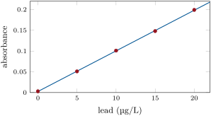
A calibration curve relates the signal $y$ of an instrument to the concentration $x$ , from standards of known concentration. The least-squares line $y = a + bx$ is the line that minimises $S = \sum (y_i - a - bx_i)^2$ ; each $e_i = y_i - a - bx_i$ is a residual.

Theorem 34.10 (Least-squares line)

With $\bar x$ , $\bar y$ the means, $S_{xx} = \sum(x_i - \bar x)^2$ and $S_{xy} = \sum(x_i - \bar x)(y_i - \bar y)$ , the least-squares line has

b = \frac{S_{xy}}{S_{xx}}, \qquad a = \bar y - b\bar x.

Proof. $S$ is a quadratic function of $a$ and $b$ . Its partial derivatives vanish at the minimum: $\partial S/\partial a = -2\sum(y_i - a - bx_i) = 0$ gives $a = \bar y - b\bar x$ ; substituting in $\partial S/\partial b = -2\sum x_i(y_i - a - bx_i) = 0$ gives $\sum x_i\bigl((y_i - \bar y) - b(x_i - \bar x)\bigr) = 0$ , that is $S_{xy} = bS_{xx}$ (since $\sum \bar x(y_i - \bar y) = \sum \bar x(x_i - \bar x) = 0$ ). The second derivatives form the matrix

\begin{pmatrix} 2n & 2\sum x_i\\ 2\sum x_i & 2\sum x_i^2\end{pmatrix},

whose diagonal is positive and whose determinant $4nS_{xx}$ is positive when the $x_i$ are not all equal: the stationary point is a minimum. ∎

Proposition 34.11 (Reading a concentration)

For $n$ standards with residual standard deviation $s_{y/x} = \sqrt{\sum e_i^2/(n-2)}$ , a sample read $m$ times with mean signal $\bar y_0$ has $x_0 = (\bar y_0 - a)/b$ and standard deviation

s_{x_0} = \frac{s_{y/x}}{b}\sqrt{\frac1m + \frac1n + \frac{(\bar y_0 - \bar y)^2}{b^2S_{xx}}},

to be used with Student’s $t$ for $n - 2$ degrees of freedom.

Proof. Admitted at this level. ∎

The three terms under the root are the scatter of the sample readings, the uncertainty of the line’s height and that of its slope; the last vanishes at the centre of the calibration range, which is where samples are best read.

Calibration of lead by graphite-furnace atomic absorption at 283.3\, nm (exercise data, used in the problem). Left: the five standards and the least-squares line. Right: the residuals, small and without pattern: a straight line is adequate. — Calibration of lead by graphite-furnace atomic absorption at $283.3\,\mathrm{nm}$ (exercise data, used in the problem). Left: the five standards and the least-squares line. Right: the residuals, small and without pattern: a straight line is adequate.

Method 34.12 (Calibrating)

Prepare five or more standards spanning the expected range, in the same matrix as the samples, and a blank.
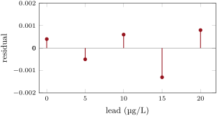
Fit the least-squares line; plot the residuals. A curved pattern means the response is not linear: narrow the range or fit a curve. One large residual points to a faulty standard.
Read the samples, preferably near the middle of the range, in replicate; compute $x_0$ and $s_{x_0}$ .
Report $x_0 \pm t\,s_{x_0}$ after correcting for every dilution, with the propagated uncertainty of the dilution added if it is not negligible.

Definition 34.13 (Standard addition)

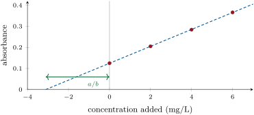
In the standard-addition method, known amounts of analyte are added to equal portions of the sample itself; the signal is plotted against the concentration added, and the concentration of the analyte in the sample is the distance from the origin to the point where the line extrapolated to zero signal crosses the axis, $a/b$ .

Method 34.14 (Standard addition)

Use it when the sample matrix changes the response (salts, acids, organic matter), so that standards in pure water would give a wrong slope.
Spike equal portions with increasing known amounts, dilute all to the same volume, measure.
Fit the line; the concentration in the measured solutions is $a/b$ ; correct for the dilution.
The response must be linear from zero: check the residuals.

Standard addition (exercise data): absorbance of a sample spiked with 0, 2, 4 and 6\, mg/ L of analyte. The line meets zero signal at -3.11\, mg/ L: the measured solution contained 3.11\, mg/ L. — Standard addition (exercise data): absorbance of a sample spiked with 0, 2, 4 and $6\,\mathrm{mg}/\mathrm{L}$ of analyte. The line meets zero signal at $-3.11\,\mathrm{mg}/\mathrm{L}$ : the measured solution contained $3.11\,\mathrm{mg}/\mathrm{L}$ .

34.5 Detection, quantification and validation

Definition 34.15 (Limits)

The limit of detection of a method is the smallest concentration whose signal can be distinguished from that of a blank with a stated small risk of a false detection; the limit of quantification is the smallest concentration that can be measured with an acceptable relative uncertainty.

Proposition 34.16 (Common estimates)

With $s_{\mathrm{blank}}$ the standard deviation of repeated blank signals and $b$ the slope of the calibration line, $x_{\mathrm{LOD}} \approx 3s_{\mathrm{blank}}/b$ and $x_{\mathrm{LOQ}} \approx 10s_{\mathrm{blank}}/b$ .

Argument. If blank signals are normal with standard deviation $s_{\mathrm{blank}}$ , a blank exceeds its mean by more than $3s_{\mathrm{blank}}$ with probability about 0.13 % (one-sided tail of the normal law beyond 3 standard deviations): calling a signal “detected” above that threshold rarely mistakes a blank for a sample. A signal $10s_{\mathrm{blank}}$ above the blank has a relative standard deviation of about 10 %, the usual threshold for a quantitative result. Dividing by $b$ converts signals into concentrations. ∎

Definition 34.17 (Validation)

Trueness is the closeness of the mean of a large number of results to the true value; their difference is the bias. Precision is the closeness of independent results to each other, expressed as a standard deviation: repeatability under the same conditions (same operator, instrument, laboratory, short time), reproducibility under changed conditions (different laboratories). Method validation is the set of experiments that establish, for a method, its trueness, precision, linearity and range, and its limits of detection and quantification.

Trueness is checked against a certified reference material or by spiking; precision by replicates in one laboratory and by comparisons between laboratories. A method can be precise but biased, every result close to the others and all of them wrong: precision is no proof of trueness.

History — Student, 1908

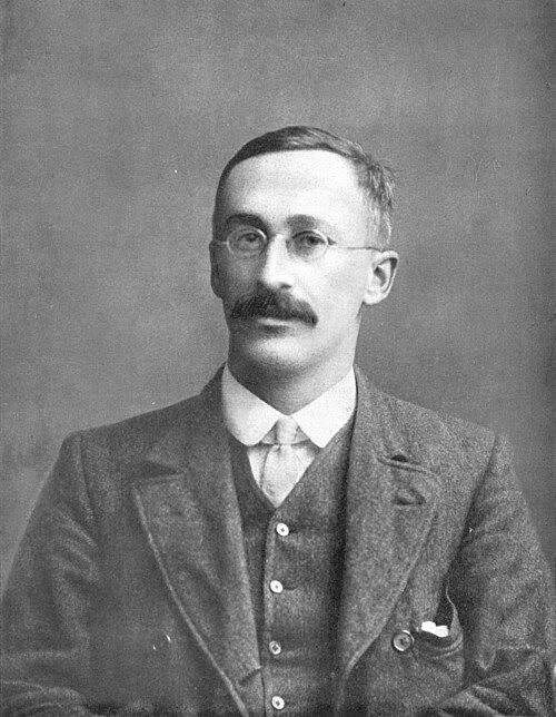
William Sealy Gosset, a chemist working for a brewery, had to judge raw materials from very few samples, far too few for the normal law. In 1908 he published the distribution of the mean divided by the sample standard deviation, under the pen name “Student” because his employer did not allow staff to publish under their names. Student’s law is used every time an analyst quotes an interval from three or four replicates. (Photograph, 1908: public domain; Wikimedia Commons.)

34.6 Exercises

Exercise 34.1 ★

Five titrations give 12.45, 12.50, 12.48, 12.52 and $12.46\,\mathrm{mL}$ . Compute the mean, the experimental standard deviation and the standard deviation of the mean.

Solution

Solution of Exercise 34.1.

$\bar V = 62.41/5 = 12.482\,\mathrm{mL}$ ; $\sum(V_i - \bar V)^2 = 0.00328$ , $s = \sqrt{0.00328/4} \approx 0.029\,\mathrm{mL}$ ; $s/\sqrt5 \approx 0.013\,\mathrm{mL}$ .

Exercise 34.2 ★

Give the 95 % confidence interval of the mean of exercise 1.

Solution

Solution of Exercise 34.2.

$t = 2.776$ for 4 degrees of freedom: $12.482 \pm 2.776 \times 0.0128$ , that is $(12.48 \pm 0.04)$ mL.

Exercise 34.3 ★

A solution is made by dissolving $m = 0.5000\,\mathrm{g}$ ( $u = 0.0002\,\mathrm{g}$ ) of a solid in a flask of $V = 250.0\,\mathrm{mL}$ ( $u = 0.15\,\mathrm{mL}$ ). Compute the relative standard uncertainty of $c = m/(MV)$ , the molar mass being exact enough.

Solution

Solution of Exercise 34.3.

The relative uncertainties of the mass and of the volume are 0.04 % and 0.06 %; combined in quadrature,

\frac{u(c)}{c} = \sqrt{\Bigl(\frac{0.0002}{0.5000}\Bigr)^2 + \Bigl(\frac{0.15}{250.0}\Bigr)^2} \approx 0.07~\%.

Exercise 34.4 ★

Fit the least-squares line through $(0, 0.02)$ , $(1, 0.21)$ , $(2, 0.39)$ , $(3, 0.62)$ .

Solution

Solution of Exercise 34.4.

$\bar x = 1.5$ , $\bar y = 0.31$ , $S_{xx} = 5$ , $S_{xy} = 0.99$ : $b = 0.198$ , $a = 0.31 - 0.198 \times 1.5 = 0.013$ .

Exercise 34.5 ★★

A certified reference solution contains $10.00\,\mathrm{mg}/\mathrm{L}$ of an element. Five analyses give a mean of $10.12\,\mathrm{mg}/\mathrm{L}$ with $s = 0.08\,\mathrm{mg}/\mathrm{L}$ . Is the method biased at the 95 % level?

Solution

Solution of Exercise 34.5.

$|10.12 - 10.00|/(0.08/\sqrt5) = 0.12/0.036 \approx 3.4 > 2.776$ : the difference is significant, the method is biased (by about $+0.12\,\mathrm{mg}/\mathrm{L}$ ).

Exercise 34.6 ★★

A concentration of hydronium ions is known with a relative standard uncertainty of 2 %. What is the standard uncertainty of the pH?

Solution

Solution of Exercise 34.6.

$\mathrm{pH} = -\log_{10}c$ , $\mathrm d\,\mathrm{pH}/\mathrm dc = -1/(c\ln10)$ : $u(\mathrm{pH}) = (u(c)/c)/\ln10 = 0.02/2.303 \approx 0.009$ .

Exercise 34.7 ★★

Ten blanks have $s = 0.0012$ absorbance units; the calibration slope is $0.0098\,\mathrm{L}/\text{µ}\mathrm{g}$ . Estimate the limits of detection and of quantification.

Solution

Solution of Exercise 34.7.

$x_{\mathrm{LOD}} = 3 \times 0.0012/0.0098 \approx 0.37\,\text{µ}\mathrm{g}/\mathrm{L}$ ; $x_{\mathrm{LOQ}} = 10 \times 0.0012/0.0098 \approx 1.2\,\text{µ}\mathrm{g}/\mathrm{L}$ .

Exercise 34.8 ★★

In the standard-addition experiment of the figure, the four portions had been made by diluting $10.0\,\mathrm{mL}$ of sample to $50.0\,\mathrm{mL}$ . Give the concentration in the sample.

Solution

Solution of Exercise 34.8.

The line gives $3.11\,\mathrm{mg}/\mathrm{L}$ in the measured solutions; the sample had been diluted fivefold: $3.11 \times 50.0/10.0 \approx 15.6\,\mathrm{mg}/\mathrm{L}$ .

Exercise 34.9 ★★

In an interlaboratory study, each laboratory obtains $s = 0.05\,\mathrm{mg}/\mathrm{L}$ on its own replicates, but the results of different laboratories scatter with $s = 0.15\,\mathrm{mg}/\mathrm{L}$ . Name the two quantities and explain the difference.

Solution

Solution of Exercise 34.9.

$0.05\,\mathrm{mg}/\mathrm{L}$ is the repeatability, $0.15\,\mathrm{mg}/\mathrm{L}$ the reproducibility. Each laboratory has its own small bias (calibration, standards, instrument); these biases differ between laboratories and add to the scatter, so reproducibility is always the larger.

Exercise 34.10 ★★★

Show that the least-squares line passes through $(\bar x, \bar y)$ and that its residuals sum to zero.

Solution

Solution of Exercise 34.10.

$\partial S/\partial a = 0$ reads $\sum(y_i - a - bx_i) = 0$ : the residuals sum to zero. Dividing by $n$ : $\bar y = a + b\bar x$ , so $(\bar x, \bar y)$ is on the line.

Exercise 34.11 ★★★

A stock solution is diluted a hundredfold either in one step ( $1.000\,\mathrm{mL}$ into $100.0\,\mathrm{mL}$ ) or in two tenfold steps ( $10.00\,\mathrm{mL}$ into $100.0\,\mathrm{mL}$ , twice). Standard uncertainties: 1 mL pipette $0.006\,\mathrm{mL}$ , 10 mL pipette $0.02\,\mathrm{mL}$ , 100 mL flask $0.08\,\mathrm{mL}$ (exercise data). Which route is more precise?

Solution

Solution of Exercise 34.11.

One step:

\sqrt{(0.006/1.000)^2 + (0.08/100.0)^2} \approx 0.61~\%.

One tenfold step:

\sqrt{(0.02/10.00)^2 + (0.08/100.0)^2} \approx 0.22~\%,

and two of them in quadrature give $0.22\sqrt2 \approx 0.30~\%$ . The two-step route is twice as precise: the small pipette dominates the one-step route.

Exercise 34.12 ★★★

The two laboratories of the opening report 9.6 and $11.2\,\text{µ}\mathrm{g}/\mathrm{L}$ with standard uncertainties 0.4 and $0.5\,\text{µ}\mathrm{g}/\mathrm{L}$ (exercise data). Are their results compatible? What does each say about the guideline value?

Solution

Solution of Exercise 34.12.

$z = 1.6/\sqrt{0.4^2 + 0.5^2} \approx 2.5 > 2$ : not compatible; one laboratory (at least) has a bias. With expanded uncertainties ( $k = 2$ ), the first gives $9.6 \pm 0.8$ , which includes 10; the second $11.2 \pm 1.0$ , entirely above 10. Before any verdict on the water, the disagreement must be resolved, for instance with a reference material.

34.7 Problem: Lead in Tap Water

Problem 34.1

Weekend problem — an atomic-absorption calibration by least squares, the concentration of a sample with its confidence interval, the dilution and the limits, and a verdict against the guideline value

Exercise data. Lead is measured by graphite-furnace atomic absorption at $283.3\,\mathrm{nm}$ . Standards ( $\text{µ}\mathrm{g}/\mathrm{L}$ ; absorbance): 0.0; 0.003, 5.0; 0.051, 10.0; 0.101, 15.0; 0.148, 20.0; 0.199. The tap water ( $50.0\,\mathrm{mL}$ ) is acidified with $0.50\,\mathrm{mL}$ of nitric acid; three readings of this solution give 0.104, 0.098 and 0.101. Ten blanks: 0.002, 0.004, 0.003, 0.001, 0.003, 0.005, 0.002, 0.003, 0.004, 0.003. Standard uncertainties of the volumes: $0.03\,\mathrm{mL}$ for 50.0 mL, $0.005\,\mathrm{mL}$ for 0.50 mL. Guideline value: $10\,\text{µ}\mathrm{g}/\mathrm{L}$ .

Part I — Calibration.

Why are the standards prepared in the same nitric acid as the samples?
Compute the slope and the intercept of the least-squares line.
Compute the five residuals.
Do the residuals show a pattern? Conclude on linearity.
Compute $s_{y/x}$ .
Why is the intercept not zero?
What does the slope measure?

Part II — The sample.

Compute the mean and the standard deviation of the three readings.
Compute the lead concentration of the measured solution.
Compute $s_{x_0}$ .
How many degrees of freedom, and which Student coefficient?
Give the 95 % interval of the concentration in the measured solution.
Why read the sample three times rather than once?

Part III — Dilution and limits.

Compute the dilution factor and the concentration in the tap water.
Propagate the uncertainty of the two volumes into the dilution factor.
Is that uncertainty significant beside the calibration one?
Compute the standard deviation of the blanks and the limit of detection.
Compute the limit of quantification.
Is the sample above the limit of quantification?

Part IV — Verdict.

Does the interval contain the guideline value?
What would a single reading of 0.104 have suggested?
What does “95 % confidence” mean here?
How could the laboratory decide more firmly?
How would it check that the method is not biased?
The guideline is provisional “on the basis of treatment performance and analytical achievability”. What does the second reason mean, in the light of this problem?
State the lead concentration of the tap water with its 95 % interval, and compare it with $10\,\text{µ}\mathrm{g}/\mathrm{L}$ .

Solution

Solution of Problem 34.1.

1. The acid changes the atomisation and the response; standards and samples must have the same matrix for the slope to apply. 2. $\bar x = 10$ , $\bar y = 0.1004$ , $S_{xx} = 250$ , $S_{xy} = 2.445$ : $b = 0.00978$ per $\text{µ}\mathrm{g}/\mathrm{L}$ , $a = 0.1004 - 0.0978 = 0.0026$ . 3. $+0.0004$ , $-0.0005$ , $+0.0006$ , $-0.0013$ , $+0.0008$ . 4. Signs alternate, no curvature: the line is adequate over 0– $20\,\text{µ}\mathrm{g}/\mathrm{L}$ . 5. $s_{y/x} = \sqrt{3.1 \times 10^{-6}/3} \approx 0.00102$ . 6. The blank (acid, water, furnace) gives a small absorbance of its own. 7. The sensitivity: absorbance per $\text{µ}\mathrm{g}/\mathrm{L}$ of lead. 8. $\bar y_0 = 0.1010$ ; $s = 0.0030$ . 9. $x_0 = (0.1010 - 0.0026)/0.00978 \approx 10.06\,\text{µ}\mathrm{g}/\mathrm{L}$ . 10. $s_{x_0} = (0.00102/0.00978)\sqrt{1/3 + 1/5 + (0.1010 - 0.1004)^2/(0.00978^2 \times 250)} \approx 0.104 \times 0.730 \approx 0.076\,\text{µ}\mathrm{g}/\mathrm{L}$ . 11. $n - 2 = 3$ ; $t = 3.182$ . 12. $10.06 \pm 3.182 \times 0.076 = (10.06 \pm 0.24)$ $\text{µ}\mathrm{g}/\mathrm{L}$ . 13. The term $1/m$ falls from 1 to $1/3$ : $s_{x_0}$ drops by about a third. 14. $f = 50.50/50.0 = 1.010$ ; $10.06 \times 1.010 \approx 10.16\,\text{µ}\mathrm{g}/\mathrm{L}$ . 15. $f = 1 + V_2/V_1$ : $u^2(f) = (u(V_2)/V_1)^2 + (V_2u(V_1)/V_1^2)^2 = (0.005/50.0)^2 + (0.50 \times 0.03/2500)^2$ , $u(f) \approx 1.0 \times 10^{-4}$ , a relative 0.01 %. 16. No: 0.01 % against $0.076/10.06 \approx 0.75~\%$ . 17. $s_{\mathrm{blank}} \approx 0.00115$ ; $x_{\mathrm{LOD}} = 3 \times 0.00115/0.00978 \approx 0.35\,\text{µ}\mathrm{g}/\mathrm{L}$ . 18. $10 \times 0.00115/0.00978 \approx 1.2\,\text{µ}\mathrm{g}/\mathrm{L}$ . 19. Yes, by far. 20. Yes: from 9.92 to $10.40\,\text{µ}\mathrm{g}/\mathrm{L}$ in the tap water. 21. $(0.104 - 0.0026)/0.00978 \times 1.010 \approx 10.5\,\text{µ}\mathrm{g}/\mathrm{L}$ , and, read alone, a confident “above the guideline” that the data do not support. 22. The rule used to build the interval captures the true value in 95 % of the series to which it is applied; it is not a probability about this one value. 23. More replicate readings and more standards near $10\,\text{µ}\mathrm{g}/\mathrm{L}$ (the terms $1/m$ and $1/n$ ), or a more sensitive method; the interval shrinks only slowly, as $1/\sqrt{\text{number}}$ . 24. By analysing a certified reference water, or by spiking the sample with a known amount of lead and checking the recovery. 25. Near $10\,\text{µ}\mathrm{g}/\mathrm{L}$ the uncertainty of routine methods is a few per cent, as here: a lower guideline value could not be checked reliably by ordinary laboratories. 26. $\boldsymbol{(10.16 \pm 0.24)}$ $\text{µ}\mathrm{g}/\mathrm{L}$ at 95 %: the interval contains $10\,\text{µ}\mathrm{g}/\mathrm{L}$ , so the measurement neither shows the water to exceed the guideline nor to meet it with a margin.

Terms defined in this chapter

See all 852 terms in the glossary