University Chemistry — Year 3 · Bachelor Year 3

13Complex Kinetics: Chains, Enzymes and Oscillations

A beaker of a stirred solution turns colourless, then amber, then blue, then colourless again, and keeps doing so for many minutes; poured into a dish, the same mixture draws spirals that rotate and travel. When Boris Belousov described such a reaction in 1951, his manuscript was rejected: a chemical system, the referee thought, cannot run back and forth, since it must go downhill towards equilibrium. It does go downhill; it simply does not go straight. This chapter treats mechanisms with many steps whose intermediates are regenerated: chain reactions and explosions, molecules that need collisions to fall apart alone, enzymes, and the oscillating reactions, with the methods that follow reactions too fast to mix by hand.

You already know

The Year 1 volume defined a reaction mechanism as a sequence of elementary steps, the rate-determining step, the pre-equilibrium and steady-state approximations, and catalysts. The Year 2 volume named the steps of a radical chain (initiation, propagation, termination), radical initiators and the kinetic chain length of a polymerisation, and fitted least-squares lines. Chapter 12 gave transition-state theory and the diffusion limit of about $10^{10}\,\mathrm{L}\,\mathrm{mol}^{-1}\,\mathrm{s}^{-1}$ .

13.1 Chain reactions

Definition 13.1 (Chain reaction, chain carrier)

A chain reaction is a reaction in which reactive intermediates, the chain carriers, are regenerated by a cycle of propagation steps, so that one initiation event converts many reactant molecules.

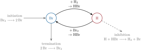
Bodenstein measured in 1906 the rate of $\ce{H2 + Br2 -> 2 HBr}$ and found a law that no single step could produce: the rate grows as $[\ce{Br2}]^{1/2}$ and falls as HBr accumulates. The mechanism was written down in 1919:

initiation	$\ce{Br2 -> 2 Br}$	$k_1$
propagation	$\ce{Br + H2 -> HBr + H}$	$k_2$
propagation	$\ce{H + Br2 -> HBr + Br}$	$k_3$
inhibition	$\ce{H + HBr -> H2 + Br}$	$k_4$
termination	$\ce{2 Br -> Br2}$	$k_{-1}$

(collisions with a third body M that carry energy in and out of the initiation and termination steps are left implicit).

Theorem 13.2 (The hydrogen–bromine rate law)

With the steady-state approximation for Br and H, the rate $v = \frac12\,\dd[\ce{HBr}]/\dd t$ of the mechanism is

v = \frac{k[\ce{H2}][\ce{Br2}]^{1/2}}{1 + k'[\ce{HBr}]/[\ce{Br2}]}, \qquad k = k_2\Bigl(\frac{k_1}{k_{-1}}\Bigr)^{1/2},\ k' = \frac{k_4}{k_3}.

Proof. Steady state for H: $k_2[\ce{Br}][\ce{H2}] = k_3[\ce{H}][\ce{Br2}] + k_4[\ce{H}][\ce{HBr}]$ . Steady state for Br: $2k_1[\ce{Br2}] - k_2[\ce{Br}][\ce{H2}] + k_3[\ce{H}][\ce{Br2}] + k_4[\ce{H}][\ce{HBr}] - 2k_{-1}[\ce{Br}]^2 = 0$ . Adding the two equations, the propagation terms cancel: $k_1[\ce{Br2}] = k_{-1}[\ce{Br}]^2$ , so $[\ce{Br}] = (k_1/k_{-1})^{1/2}[\ce{Br2}]^{1/2}$ . Then $[\ce{H}] = k_2[\ce{Br}][\ce{H2}]/(k_3[\ce{Br2}] + k_4[\ce{HBr}])$ and

\frac{\dd[\ce{HBr}]}{\dd t} = k_2[\ce{Br}][\ce{H2}] + k_3[\ce{H}][\ce{Br2}] - k_4[\ce{H}][\ce{HBr}] = 2k_3[\ce{H}][\ce{Br2}] = \frac{2k_2[\ce{Br}][\ce{H2}]}{1 + (k_4/k_3)[\ce{HBr}]/[\ce{Br2}]},

using the first equation; substituting $[\ce{Br}]$ gives the result. ∎

The propagation cycle of the hydrogen–bromine chain: each turn consumes one H2 and one Br2, makes two HBr and gives back the bromine atom that started it. Initiation feeds the cycle with carriers, termination removes them; the inhibition step turns an H atom back into Br at the cost of an HBr already made. — The propagation cycle of the hydrogen–bromine chain: each turn consumes one $\ce{H2}$ and one $\ce{Br2}$ , makes two HBr and gives back the bromine atom that started it. Initiation feeds the cycle with carriers, termination removes them; the inhibition step turns an H atom back into Br at the cost of an HBr already made.

The hydrogen–bromine mechanism integrated step by step (model rate constants, reduced units, k' = 0.1): conversion against time (left), and the rate 1/2 [ HBr]/ t of the full mechanism compared with the steady-state law (right). After an induction period, during which the bromine atoms build up, the two coincide to better than 1 %. — The hydrogen–bromine mechanism integrated step by step (model rate constants, reduced units, $k' = 0.1$ ): conversion against time (left), and the rate $\frac12\dd[\ce{HBr}]/\dd t$ of the full mechanism compared with the steady-state law (right). After an induction period, during which the bromine atoms build up, the two coincide to better than 1 %.

Method 13.3 (The rate law of a chain mechanism)

Write a steady-state equation for each chain carrier.
Add them: the propagation steps, which only exchange one carrier for another, cancel, leaving initiation equal to termination; this gives the carrier concentration.
Use one carrier’s equation to express the other carriers.
Write the rate of formation of a product from the propagation steps.

The number of propagation cycles per initiation event, here $v/k_1[\ce{Br2}]$ , is the kinetic chain length of the Year 2 volume; for the hydrogen–bromine reaction it is of the order of $10^3$ to $10^6$ depending on the conditions. Inhibition by the product explains why the rate falls faster than the reactants are consumed.

13.2 Branching chains and explosions

Definition 13.4 (Chain branching, explosion limits)

Chain branching is a propagation step that produces more chain carriers than it consumes, such as $\ce{H + O2 -> OH + O}$ , which turns one carrier into two. The explosion limits of a mixture are the pressures, at a given temperature, at which its slow reaction turns into an explosion.

Proposition 13.5 (Branching criterion)

Let carriers be created at the rate $v_i$ , multiply by branching with the rate constant $f$ and disappear by termination with the rate constant $g$ : $\dd n/\dd t = v_i + (f - g)n$ . If $f < g$ , $n$ tends to the steady value $v_i/(g - f)$ ; if $f > g$ , $n$ grows exponentially and the reaction explodes.

Proof. The linear equation has the solution $n(t) = \frac{v_i}{g - f}\bigl(1 - \eu^{-(g - f)t}\bigr)$ , which tends to $v_i/(g - f)$ when $g > f$ ; when $f > g$ the exponent is positive and $n$ grows as $\eu^{(f - g)t}$ without bound (until the reactants run out). ∎

For hydrogen–oxygen mixtures at a few hundred degrees, $f$ grows with the pressure (it is proportional to $[\ce{O2}]$ ), termination at the walls of the vessel is fast at low pressure (the radicals diffuse there easily), and termination by three-body collisions ( $\ce{H + O2 + M -> HO2 + M}$ ) grows as the square of the pressure. Branching wins between a first limit, set by the walls, and a second limit, set by three-body termination; at still higher pressure a third limit appears where the heat released can no longer escape. The last is a thermal explosion, driven by the exponential growth of the rate with temperature rather than by branching; most industrial explosions are of that kind.

13.3 Unimolecular reactions

A molecule such as cyclopropane isomerises alone, with first-order kinetics at ordinary pressures; yet at low pressure the rate constant falls. The energy needed comes from collisions.

Definition 13.6 (Lindemann mechanism, fall-off region)

The Lindemann mechanism of a unimolecular reaction is the sequence $\mathrm{A + M \rightleftharpoons A^* + M}$ ( $k_1$ , $k_{-1}$ ), activation and deactivation by collision with any molecule M, followed by $\mathrm{A^* \to P}$ ( $k_2$ ). The fall-off region is the range of pressures where the observed first-order rate constant falls from its high-pressure value towards second-order behaviour.

Theorem 13.7 (Lindemann rate constant)

With the steady-state approximation for $\mathrm{A^*}$ , $v = k_{\mathrm{uni}}[\mathrm A]$ with

k_{\mathrm{uni}} = \frac{k_1k_2[\mathrm M]}{k_{-1}[\mathrm M] + k_2},

which tends to $k_\infty = k_1k_2/k_{-1}$ at high pressure (first order) and to $k_1[\mathrm M]$ at low pressure (second order); it is $k_\infty/2$ at $[\mathrm M]_{1/2} = k_2/k_{-1}$ .

Proof. $\dd[\mathrm{A^*}]/\dd t = k_1[\mathrm A][\mathrm M] - k_{-1}[\mathrm{A^*}][\mathrm M] - k_2[\mathrm{A^*}] = 0$ gives $[\mathrm{A^*}] = k_1[\mathrm A][\mathrm M]/(k_{-1}[\mathrm M] + k_2)$ and $v = k_2[\mathrm{A^*}]$ . If $k_{-1}[\mathrm M] \gg k_2$ , deactivation outruns reaction and $\mathrm{A^*}$ is in pre-equilibrium: $k_{\mathrm{uni}} \to k_1k_2/k_{-1}$ . If $k_{-1}[\mathrm M] \ll k_2$ , every activated molecule reacts and activation is rate-determining: $k_{\mathrm{uni}} \to k_1[\mathrm M]$ . ∎

The Lindemann fall-off curve (model constants): first order with the limiting constant k_∈fty at high pressure, second order (k_1[ M]) at low pressure, and half of k_∈fty at [ M]_1/2 = k_2/k_-1. Real fall-off curves are broader: the rate constant k_2 of an energised molecule grows with its energy. — The Lindemann fall-off curve (model constants): first order with the limiting constant $k_\infty$ at high pressure, second order ( $k_1[\mathrm M]$ ) at low pressure, and half of $k_\infty$ at $[\mathrm M]_{1/2} = k_2/k_{-1}$ . Real fall-off curves are broader: the rate constant $k_2$ of an energised molecule grows with its energy.

13.4 Enzyme kinetics

Definition 13.8 (Enzyme, active site, enzyme–substrate complex)

An enzyme is a biological catalyst, almost always a protein, that speeds up a specific reaction of its substrate. The active site is the pocket of the enzyme where the substrate binds and reacts; the bound species is the enzyme–substrate complex ES.

Definition 13.9 (Michaelis constant, maximum rate, catalytic and specificity constants)

For the mechanism $\mathrm{E + S \rightleftharpoons ES \to E + P}$ ( $k_1$ , $k_{-1}$ , $k_2$ ) at total enzyme concentration $[\mathrm E]_0$ , the catalytic constant is $k_{\mathrm{cat}} = k_2$ , the maximum rate is $V_{\max} = k_{\mathrm{cat}}[\mathrm E]_0$ , the Michaelis constant is $K_M = (k_{-1} + k_2)/k_1$ , and the specificity constant is $k_{\mathrm{cat}}/K_M$ .

Theorem 13.10 (Michaelis–Menten equation)

When $[\mathrm S] \gg [\mathrm E]_0$ and ES is in a steady state, the initial rate of formation of the product is

v = \frac{V_{\max}[\mathrm S]}{K_M + [\mathrm S]} .

This statement is the Michaelis–Menten equation.

Proof. Steady state: $k_1[\mathrm E][\mathrm S] = (k_{-1} + k_2)[\mathrm{ES}]$ , and $[\mathrm E] = [\mathrm E]_0 - [\mathrm{ES}]$ (the free substrate is practically all the substrate since $[\mathrm S] \gg [\mathrm E]_0$ ). Hence $[\mathrm{ES}] = [\mathrm E]_0[\mathrm S]/(K_M + [\mathrm S])$ and $v = k_2[\mathrm{ES}]$ . ∎

Remark 13.11

Michaelis and Menten (1913) assumed instead a rapid pre-equilibrium of E, S and ES; the same equation follows with $K_M$ replaced by the dissociation constant $k_{-1}/k_1$ , the limit of $K_M$ when $k_2 \ll k_{-1}$ . The catalytic constant is what biochemists call the turnover number of the enzyme: the number of substrate molecules one active site converts per second when saturated.

At $[\mathrm S] = K_M$ the rate is $V_{\max}/2$ ; at $[\mathrm S] \ll K_M$ it is $(k_{\mathrm{cat}}/K_M)[\mathrm E]_0[\mathrm S]$ : the specificity constant is the second-order rate constant of the free enzyme with its substrate, and it cannot exceed the rate at which they meet, the diffusion limit of Chapter 12. A few enzymes come close; the “average” enzyme, in a survey of several thousand, has $k_{\mathrm{cat}}/K_M$ of about $10^5$ $\mathrm{L}\,\mathrm{mol}^{-1}\,\mathrm{s}^{-1}$ , some four orders of magnitude below.

Proposition 13.12 (Lineweaver–Burk form)

The Michaelis–Menten equation is equivalent to

\frac1v = \frac{1}{V_{\max}} + \frac{K_M}{V_{\max}}\,\frac{1}{[\mathrm S]},

a straight line of $1/v$ against $1/[\mathrm S]$ with intercept $1/V_{\max}$ , slope $K_M/V_{\max}$ , and intercept $-1/K_M$ on the $1/[\mathrm S]$ axis.

Proof. Invert: $1/v = (K_M + [\mathrm S])/(V_{\max}[\mathrm S])$ . At $1/v = 0$ , $1/[\mathrm S] = -1/K_M$ . ∎

Method 13.13 ( $K_M$ and $V_{\max}$ by nonlinear least squares)

Measure initial rates at substrate concentrations spread from about $K_M/5$ to $10K_M$ .
Fit $v = V_{\max}[\mathrm S]/(K_M + [\mathrm S])$ directly, by minimising $\sum(v_i - v(\mathrm S_i))^2$ (iteratively, starting from the values of a Lineweaver–Burk line); the standard errors come from the residuals and the sensitivity of $v$ to each parameter.
Use the Lineweaver–Burk plot only to see the pattern: inverting small rates magnifies their errors, so the least-squares line through $1/v$ is dominated by the least precise points, and its parameters are biased.

Definition 13.14 (Inhibition)

An inhibitor I binds the enzyme reversibly. In competitive inhibition it binds only the free enzyme, at the active site, with the inhibition constant $K_i$ (dissociation constant of EI); in uncompetitive inhibition it binds only ES, with the constant $K_i'$ ; in mixed inhibition it binds both.

Proposition 13.15 (Inhibited rate laws)

With $\alpha = 1 + [\mathrm I]/K_i$ and $\alpha' = 1 + [\mathrm I]/K_i'$ , the rate keeps the Michaelis–Menten form $v = V^{\mathrm{app}}[\mathrm S]/(K_M^{\mathrm{app}} + [\mathrm S])$ with: competitive, $K_M^{\mathrm{app}} = \alpha K_M$ , $V^{\mathrm{app}} = V_{\max}$ ; uncompetitive, $K_M^{\mathrm{app}} = K_M/\alpha'$ , $V^{\mathrm{app}} = V_{\max}/\alpha'$ ; mixed, $K_M^{\mathrm{app}} = \alpha K_M/\alpha'$ , $V^{\mathrm{app}} = V_{\max}/\alpha'$ .

Proof. Mixed case (the others are its limits $K_i' \to \infty$ and $K_i \to \infty$ ): the enzyme is shared among E, EI, ES and ESI with $[\mathrm{EI}] = [\mathrm E][\mathrm I]/K_i$ , $[\mathrm{ESI}] = [\mathrm{ES}][\mathrm I]/K_i'$ and the steady state $[\mathrm E][\mathrm S] = K_M[\mathrm{ES}]$ . So $[\mathrm E]_0 = [\mathrm E]\alpha + [\mathrm{ES}]\alpha' = [\mathrm{ES}](\alpha K_M/[\mathrm S] + \alpha')$ and $v = k_2[\mathrm{ES}] = V_{\max}[\mathrm S]/(\alpha K_M + \alpha'[\mathrm S])$ ; dividing numerator and denominator by $\alpha'$ gives the stated form. ∎

Method 13.16 (Recognising the type of inhibition)

Measure $v([\mathrm S])$ at several inhibitor concentrations and draw the Lineweaver–Burk lines.
Lines meeting on the $1/v$ axis (same $V_{\max}$ ): competitive; a large excess of substrate overcomes the inhibitor.
Parallel lines (slope $K_M/V_{\max}$ unchanged): uncompetitive.
Lines meeting to the left of the $1/v$ axis: mixed.
Obtain $K_i$ by fitting the apparent constants against $[\mathrm I]$ : for a competitive inhibitor $K_M^{\mathrm{app}} = K_M + (K_M/K_i)[\mathrm I]$ , a straight line.

Michaelis–Menten kinetics with K_M = 0.80\, mM and V_ = 0.50\, µ M\, s-1 (model): no inhibitor (black), a competitive inhibitor at [ I] = 2K_i (blue, K_M tripled, same V_) and an uncompetitive one at [ I] = K_i' (red, K_M and V_ halved). Right: the Lineweaver–Burk lines; the competitive line meets the uninhibited one on the 1/v axis, the uncompetitive one is parallel to it (1/[ S] in mM-1, 1/v in s\, µ M-1). — Michaelis–Menten kinetics with $K_M = 0.80\,\mathrm{mM}$ and $V_{\max} = 0.50\,\text{µ}\mathrm{M}\,\mathrm{s}^{-1}$ (model): no inhibitor (black), a competitive inhibitor at $[\mathrm I] = 2K_i$ (blue, $K_M$ tripled, same $V_{\max}$ ) and an uncompetitive one at $[\mathrm I] = K_i'$ (red, $K_M$ and $V_{\max}$ halved). Right: the Lineweaver–Burk lines; the competitive line meets the uninhibited one on the $1/v$ axis, the uncompetitive one is parallel to it ( $1/[\mathrm S]$ in $\mathrm{mM}^{-1}$ , $1/v$ in $\mathrm{s}\,\text{µ}\mathrm{M}^{-1}$ ).

13.5 Autocatalysis, oscillations and fast reactions

Definition 13.17 (Autocatalytic reaction)

An autocatalytic reaction is one in which a product catalyses its own formation, as in $\mathrm{A + X \to 2\,X}$ .

Proposition 13.18 (Logistic law)

For $\mathrm{A + X \to 2\,X}$ with rate constant $k$ and initial concentrations $a_0$ and $x_0$ , with $N = a_0 + x_0$ ,

x(t) = \frac{N}{1 + (N/x_0 - 1)\eu^{-kNt}},

an S-shaped curve that reaches half its final value at $t_{1/2} = \ln(N/x_0 - 1)/kN$ .

Proof. $\dd x/\dd t = kx(N - x)$ , since $a = N - x$ . Separating, $\frac{\dd x}{x(N - x)} = \frac1N\bigl(\frac1x + \frac{1}{N - x}\bigr)\dd x = k\,\dd t$ , so $\ln\frac{x}{N - x} = kNt + \ln\frac{x_0}{N - x_0}$ , which rearranges into the stated form; $x = N/2$ when $(N/x_0 - 1)\eu^{-kNt} = 1$ . ∎

Definition 13.19 (Oscillating reaction, limit cycle)

An oscillating reaction is one in which the concentrations of intermediates rise and fall periodically while the overall reaction proceeds towards equilibrium. A limit cycle is a closed trajectory in the space of concentrations towards which neighbouring trajectories converge, so that the oscillation has an amplitude independent of the starting point.

Theorem 13.20 (Lotka–Volterra model)

For the autocatalytic scheme $\mathrm{A + X \to 2\,X}$ , $\mathrm{X + Y \to 2\,Y}$ , $\mathrm{Y \to B}$ with A held constant, the concentrations obey $\dot x = x(a - by)$ , $\dot y = y(dx - c)$ with positive constants, and the quantity

V = dx - c\ln x + by - a\ln y

is constant along each trajectory: the trajectories are closed curves around the steady state $(c/d, a/b)$ , and the concentrations oscillate with an amplitude fixed by the starting point.

Proof. $\dot V = (d - c/x)\dot x + (b - a/y)\dot y = (dx - c)(a - by) + (by - a)(dx - c) = 0$ . $V$ is a sum of two convex functions with a single minimum at $(c/d, a/b)$ , so its level curves are closed curves around that point; a trajectory stays on one of them and, the velocity never vanishing elsewhere, goes round it periodically. ∎

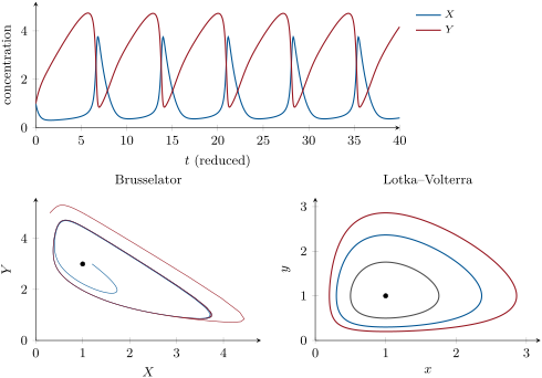
The Lotka–Volterra oscillations are fragile: every starting point gives its own orbit, and any perturbation moves the system to another. Real chemical oscillators have a limit cycle, which needs a nonlinearity that destabilises the steady state.

Proposition 13.21 (Instability of the Brusselator)

The model $\dot X = A - (B + 1)X + X^2Y$ , $\dot Y = BX - X^2Y$ (reduced concentrations, $A$ and $B$ held constant) has the single steady state $(A, B/A)$ , which is stable if $B < 1 + A^2$ and unstable if $B > 1 + A^2$ ; the system then settles on a limit cycle.

Proof. Setting both derivatives to zero: $BX = X^2Y$ gives $XY = B$ , and then $A - X = 0$ . The Jacobian matrix at $(A, B/A)$ is

\begin{pmatrix} -(B + 1) + 2XY & X^2 \\ B - 2XY & -X^2 \end{pmatrix} = \begin{pmatrix} B - 1 & A^2 \\ -B & -A^2 \end{pmatrix},

with trace $B - 1 - A^2$ and determinant $A^2 > 0$ . Small deviations evolve as $\eu^{\lambda t}$ with $\lambda$ the eigenvalues, whose product is the determinant (positive) and whose sum is the trace: both have negative real parts when the trace is negative, positive real parts when it is positive. The existence of the limit cycle for $B > 1 + A^2$ (the trajectories being confined to a bounded region) is admitted. ∎

Method 13.22 (The linear stability of a steady state)

Find the steady state by setting all time derivatives to zero.
Compute the Jacobian matrix of partial derivatives of the rates there.
For two variables: stable if the trace is negative and the determinant positive; an unstable state with complex eigenvalues ( $\mathrm{tr}^2 < 4\det$ ) gives growing oscillations, a candidate limit cycle.

Top: the Brusselator (A = 1, B = 3 > 1 + A2) settles into sustained oscillations of period 7.2 (reduced time). Bottom left: two trajectories, one starting near the unstable steady state (dot) and one far outside, wind onto the same limit cycle. Bottom right: Lotka–Volterra orbits, each fixed by its starting point, around the steady state (dot). — Top: the Brusselator ( $A = 1$ , $B = 3 > 1 + A^2$ ) settles into sustained oscillations of period 7.2 (reduced time). Bottom left: two trajectories, one starting near the unstable steady state (dot) and one far outside, wind onto the same limit cycle. Bottom right: Lotka–Volterra orbits, each fixed by its starting point, around the steady state (dot).

The Belousov–Zhabotinsky reaction, the oxidation of malonic acid by bromate catalysed by cerium or by a ferroin indicator, runs through such a cycle: an autocatalytic production of $\ce{HBrO2}$ switches on when bromide falls below a threshold, oxidises the catalyst (the colour change), and is switched off when the oxidised catalyst regenerates bromide. Unstirred, in a thin layer, the oscillation propagates as waves.

Spiral waves of the Belousov–Zhabotinsky reaction in a thin layer of solution: each blue front is a wave of oxidation of the catalyst, which travels into the reduced (red) medium and cannot re-enter the region it just left.

Definition 13.23 (Relaxation method, chemical relaxation time)

A relaxation method perturbs a system at equilibrium suddenly (by a jump of temperature, pressure or electric field) and follows its return to the new equilibrium. For a small perturbation the deviation decays exponentially, with the chemical relaxation time $\tau$ .

Proposition 13.24 (Relaxation time of an association)

For $\mathrm{A + B \rightleftharpoons C}$ ( $k_1$ , $k_{-1}$ ), after a small perturbation,

\frac1\tau = k_1([\mathrm A]_e + [\mathrm B]_e) + k_{-1} .

Proof. Write $[\mathrm C] = [\mathrm C]_e + x$ , $[\mathrm A] = [\mathrm A]_e - x$ , $[\mathrm B] = [\mathrm B]_e - x$ . Then $\dot x = k_1([\mathrm A]_e - x)([\mathrm B]_e - x) - k_{-1}([\mathrm C]_e + x)$ ; the terms without $x$ cancel at equilibrium, and dropping $x^2$ : $\dot x = -[k_1([\mathrm A]_e + [\mathrm B]_e) + k_{-1}]x$ . ∎

Measuring $\tau$ at several concentrations gives a line of $1/\tau$ against $[\mathrm A]_e + [\mathrm B]_e$ whose slope is $k_1$ and intercept $k_{-1}$ : both constants from experiments on a system that never leaves equilibrium by more than a few per cent. Manfred Eigen measured in this way the fastest reactions in solution, among them the neutralisation of $\ce{H3O+}$ by $\ce{OH-}$ .

Relaxation of A + B C after a temperature jump that lowered its equilibrium constant by 5 % (model: k_1 = 1.0 × 108\, L\, mol-1\, s-1, k_-1 = 1.0 × 103\, s-1, 1.0 × 10-4\, mol/ L of A and B in all): the full rate equation and the exponential with 1/ = k_1([ A]_e + [ B]_e) + k_-1 coincide. — Relaxation of $\mathrm{A + B \rightleftharpoons C}$ after a temperature jump that lowered its equilibrium constant by 5 % (model: $k_1 = 1.0 \times 10^{8}\,\mathrm{L}\,\mathrm{mol}^{-1}\,\mathrm{s}^{-1}$ , $k_{-1} = 1.0 \times 10^{3}\,\mathrm{s}^{-1}$ , $1.0 \times 10^{-4}\,\mathrm{mol}/\mathrm{L}$ of A and B in all): the full rate equation and the exponential with $1/\tau = k_1([\mathrm A]_e + [\mathrm B]_e) + k_{-1}$ coincide.

Definition 13.25 (Stopped flow, flash photolysis)

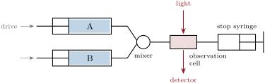
The stopped-flow method mixes two reactant solutions in about a millisecond by driving them through a mixer into an observation cell, then stops the flow and records the absorbance or fluorescence. Flash photolysis creates a reactive species by a short intense light pulse and follows its reactions with a second, delayed light beam.

A stopped-flow apparatus. The drive pushes two syringes; the solutions meet in the mixer and fill the observation cell within about a millisecond; the plunger of the stop syringe hits a block, the flow stops, and the detector records the reaction of the freshly mixed solution.

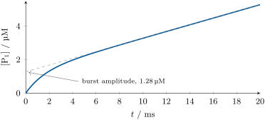
A stopped-flow burst trace (data of the weekend problem): the first product of a two-step enzyme appears in a fast burst followed by a straight line; the dashed line extrapolates the steady state back to t = 0. — A stopped-flow burst trace (data of the weekend problem): the first product of a two-step enzyme appears in a fast burst followed by a straight line; the dashed line extrapolates the steady state back to $t = 0$ .

In the lab — A stopped-flow measurement

The two syringes are filled with enzyme and substrate solutions in the same buffer, thermostated, and fired several times to flush the cell before the recorded shots; each trace is averaged over five to ten shots. The dead time, the age of the mixture when observation starts, is measured once with a reaction of known rate.

Safety

Bromine: a volatile, dense red-brown liquid; fatal if inhaled, causes severe burns, very toxic to aquatic life. Handled only in a fume hood, with gloves and face protection; a solution of sodium thiosulfate is kept at hand to reduce spills.

History — Bodenstein and Belousov

Max Bodenstein and Samuel Lind measured the hydrogen–bromine rate law in 1906; Jens Christiansen, Karl Herzfeld and Michael Polanyi explained it in 1919 with the chain mechanism of this chapter. Boris Belousov, a biochemist in Moscow, found his oscillating reaction around 1951 while looking for a chemical model of a metabolic cycle; his manuscript was rejected, and only a short abstract appeared in 1959. Anatol Zhabotinsky took up the reaction in the 1960s and explained it; the full mechanism was worked out in the early 1970s.

13.6 Exercises

Exercise 13.1 ★

For the chain $\ce{Cl2 -> 2 Cl}$ , $\ce{Cl + H2 -> HCl + H}$ , $\ce{H + Cl2 -> HCl + Cl}$ , $\ce{2 Cl -> Cl2}$ , name each step and the chain carriers, and write the overall reaction.

Solution

Solution of Exercise 13.1.

$\ce{Cl2 -> 2 Cl}$ : initiation; $\ce{Cl + H2 -> HCl + H}$ and $\ce{H + Cl2 -> HCl + Cl}$ : propagation; $\ce{2 Cl -> Cl2}$ : termination. Carriers: Cl and H. Overall (sum of the two propagation steps): $\ce{H2 + Cl2 -> 2 HCl}$ .

Exercise 13.2 ★

A Lindemann system has $k_2 = 1.0 \times 10^{7}\,\mathrm{s}^{-1}$ and $k_{-1} = 1.0 \times 10^{10}\,\mathrm{L}\,\mathrm{mol}^{-1}\,\mathrm{s}^{-1}$ (data of the exercise). Compute $[\mathrm M]_{1/2}$ and the corresponding pressure at $750\,\mathrm{K}$ .

Solution

Solution of Exercise 13.2.

$[\mathrm M]_{1/2} = k_2/k_{-1} = 1.0 \times 10^{-3}\,\mathrm{mol}/\mathrm{L} = 1.0\,\mathrm{mol}/\mathrm{m}^{3}$ ; $p = cRT = 1.0 \times 8.314 \times 750 = 6.2\,\mathrm{kPa}$ .

Exercise 13.3 ★

Express $v/V_{\max}$ at $[\mathrm S] = K_M$ , $3K_M$ and $9K_M$ . What concentration gives 90 % of $V_{\max}$ ?

Solution

Solution of Exercise 13.3.

$v/V_{\max} = [\mathrm S]/(K_M + [\mathrm S])$ : $\frac12$ , $\frac34$ , $\frac{9}{10}$ . 90 % of $V_{\max}$ needs $[\mathrm S] = 9K_M$ .

Exercise 13.4 ★

An enzyme has $k_{\mathrm{cat}} = 100\,\mathrm{s}^{-1}$ and $K_M = 0.80\,\mathrm{mM}$ . Compute its specificity constant and compare it with the diffusion limit in water, $7.4 \times 10^{9}\,\mathrm{L}\,\mathrm{mol}^{-1}\,\mathrm{s}^{-1}$ , and with the typical $10^5$ $\mathrm{L}\,\mathrm{mol}^{-1}\,\mathrm{s}^{-1}$ .

Solution

Solution of Exercise 13.4.

$k_{\mathrm{cat}}/K_M = 100/0.80 \times 10^{-3} = 1.25 \times 10^{5}\,\mathrm{L}\,\mathrm{mol}^{-1}\,\mathrm{s}^{-1}$ : some 60 000 times below the diffusion limit, and close to the typical value.

Exercise 13.5 ★★

The decomposition $\ce{CH3CHO -> CH4 + CO}$ is proposed to run by: $\ce{CH3CHO -> CH3 + CHO}$ ( $k_1$ ); $\ce{CH3 + CH3CHO -> CH4 + CH3CO}$ ( $k_2$ ); $\ce{CH3CO -> CH3 + CO}$ ( $k_3$ ); $\ce{2 CH3 -> C2H6}$ ( $k_4$ ). Show that the rate of formation of methane is $k_2(k_1/2k_4)^{1/2}[\ce{CH3CHO}]^{3/2}$ .

Solution

Solution of Exercise 13.5.

Steady state for $\ce{CH3CO}$ : $k_2[\ce{CH3}][\ce{CH3CHO}] = k_3[\ce{CH3CO}]$ . Steady state for $\ce{CH3}$ : $k_1[\ce{CH3CHO}] - k_2[\ce{CH3}][\ce{CH3CHO}] + k_3[\ce{CH3CO}] - 2k_4[\ce{CH3}]^2 = 0$ . Adding: $k_1[\ce{CH3CHO}] = 2k_4[\ce{CH3}]^2$ , so $[\ce{CH3}] = (k_1/2k_4)^{1/2}[\ce{CH3CHO}]^{1/2}$ , and $\dd[\ce{CH4}]/\dd t = k_2[\ce{CH3}][\ce{CH3CHO}] = k_2(k_1/2k_4)^{1/2}[\ce{CH3CHO}]^{3/2}$ .

Exercise 13.6 ★★

Starting from equal concentrations of $\ce{H2}$ and $\ce{Br2}$ , with $k' = 0.10$ , by what factor has the rate fallen when half the bromine is consumed? How much of the fall is due to inhibition?

Solution

Solution of Exercise 13.6.

At half conversion $[\ce{H2}] = [\ce{Br2}] = \frac12$ , $[\ce{HBr}] = 1$ (relative units): $v/v_0 = \frac12 \times (\frac12)^{1/2}/(1 + 0.10 \times 1/0.5) = 0.354/1.2 = 0.29$ . Without inhibition it would be 0.354: inhibition divides the rate by a further 1.2.

Exercise 13.7 ★★

In a model hydrogen–oxygen mixture (data of the exercise), branching has the rate constant $f = 1000\,p$ , wall termination $6000/p$ and three-body termination $10\,p^2$ , all in $\mathrm{s}^{-1}$ with $p$ in kPa. Find the pressure range in which the mixture explodes.

Solution

Solution of Exercise 13.7.

Explosion when $1000p > 6000/p + 10p^2$ , i.e. $10p^3 - 1000p^2 + 6000 < 0$ , whose positive roots are 2.48 and $99.9\,\mathrm{kPa}$ : the mixture explodes between about 2.5 and $100\,\mathrm{kPa}$ (first and second limits of the model).

Exercise 13.8 ★★

Initial rates are $0.20\,\text{µ}\mathrm{M}\,\mathrm{s}^{-1}$ at $[\mathrm S] = 0.50\,\mathrm{mM}$ and $0.40\,\text{µ}\mathrm{M}\,\mathrm{s}^{-1}$ at $2.0\,\mathrm{mM}$ . Find $K_M$ and $V_{\max}$ .

Solution

Solution of Exercise 13.8.

$1/v = 1/V_{\max} + (K_M/V_{\max})/[\mathrm S]$ : $5.0 = 1/V_{\max} + 2.0K_M/V_{\max}$ and $2.5 = 1/V_{\max} + 0.5K_M/V_{\max}$ . Subtracting: $K_M/V_{\max} = 1.667\,\mathrm{s}\,\mathrm{mM}\,\text{µ}\mathrm{M}^{-1}$ , then $1/V_{\max} = 1.667$ : $V_{\max} = 0.60\,\text{µ}\mathrm{M}\,\mathrm{s}^{-1}$ , $K_M = 1.0\,\mathrm{mM}$ .

Exercise 13.9 ★★

With $50\,\text{µ}\mathrm{M}$ of an inhibitor, the Lineweaver–Burk line of an enzyme ( $K_M = 0.80\,\mathrm{mM}$ ) meets the uninhibited one on the $1/v$ axis and crosses the $1/[\mathrm S]$ axis at $-0.417\,\mathrm{mM}^{-1}$ . Identify the type of inhibition and compute $K_i$ .

Solution

Solution of Exercise 13.9.

Same intercept on the $1/v$ axis: competitive. $K_M^{\mathrm{app}} = 1/0.417 = 2.40\,\mathrm{mM} = 3K_M$ , so $1 + 50/K_i = 3$ and $K_i = 25\,\text{µ}\mathrm{M}$ .

Exercise 13.10 ★★★

For $\mathrm{A + X \to 2\,X}$ with $k = 0.50\,\mathrm{L}\,\mathrm{mol}^{-1}\,\mathrm{s}^{-1}$ , $a_0 = 1.00\,\mathrm{mol}/\mathrm{L}$ and $x_0 = 0.010\,\mathrm{mol}/\mathrm{L}$ , compute the time at which half the final amount of X is present, and the time of maximum rate.

Solution

Solution of Exercise 13.10.

$N = 1.01\,\mathrm{mol}/\mathrm{L}$ : $t_{1/2} = \ln(1.01/0.010 - 1)/(0.50 \times 1.01) = \ln100/0.505 = 9.1\,\mathrm{s}$ . The rate $kx(N - x)$ is largest at $x = N/2$ : the same instant, the inflexion of the S curve.

Exercise 13.11 ★★★

For the Brusselator with $A = 1$ , compute the eigenvalues of the Jacobian at the steady state for $B = 1.5$ and $B = 2.5$ , and describe the behaviour near the steady state in each case.

Solution

Solution of Exercise 13.11.

Trace $B - 2$ , determinant 1. $B = 1.5$ : $\lambda = -0.25 \pm 0.968\iu$ , a stable focus (damped oscillations towards the steady state). $B = 2.5$ : $\lambda = 0.25 \pm 0.968\iu$ , an unstable focus: oscillations grow until they reach the limit cycle.

Exercise 13.12 ★★★

For $\mathrm{A + B \rightleftharpoons C}$ with $k_1 = 1.0 \times 10^{8}\,\mathrm{L}\,\mathrm{mol}^{-1}\,\mathrm{s}^{-1}$ and $k_{-1} = 1.0 \times 10^{3}\,\mathrm{s}^{-1}$ , and $[\mathrm A]_e = [\mathrm B]_e = 2.70 \times 10^{-5}\,\mathrm{mol}/\mathrm{L}$ , compute $\tau$ . How would you obtain both rate constants from relaxation measurements alone?

Solution

Solution of Exercise 13.12.

$1/\tau = 1.0 \times 10^{8} \times 5.40 \times 10^{-5} + 1.0 \times 10^{3} = 6.4 \times 10^{3}\,\mathrm{s}^{-1}$ , $\tau = 156\,\text{µ}\mathrm{s}$ . Measure $\tau$ at several total concentrations: $1/\tau$ against $[\mathrm A]_e + [\mathrm B]_e$ is a straight line of slope $k_1$ and intercept $k_{-1}$ .

13.7 Problem: An Enzyme, an Inhibitor and a Dose

Problem 13.1

Weekend problem — an enzyme, an inhibitor and a dose: the Michaelis–Menten parameters by least squares, the inhibition constant of a competitive inhibitor, the activity left at a given dose, and a stopped-flow burst

An enzyme ( $[\mathrm E]_0 = 5.0\,\mathrm{nM}$ in the assays) hydrolyses its substrate; initial rates (data of the problem):

$[\mathrm S]$ / mM	0.10	0.20	0.40	0.80	1.60	3.20	6.40
$v$ / $\text{µ}\mathrm{M}\,\mathrm{s}^{-1}$	0.0566	0.0981	0.169	0.247	0.340	0.397	0.447

In the presence of an inhibitor, fits of the same kind give $V_{\max}$ unchanged and the apparent $K_M$ : 0.79, 1.47, 2.38 and $4.02\,\mathrm{mM}$ at $[\mathrm I] = 0$ , 20, 50 and $100\,\text{µ}\mathrm{M}$ . A stopped-flow experiment with $[\mathrm E]_0 = 2.0\,\text{µ}\mathrm{M}$ and saturating substrate gives the burst trace of the figure of section 5 (a burst of $1.28\,\text{µ}\mathrm{M}$ with rate constant $625\,\mathrm{s}^{-1}$ , then $200\,\text{µ}\mathrm{M}\,\mathrm{s}^{-1}$ ).

Part I — $K_M$ and $V_{\max}$ .

Why are initial rates used?
Draw the Lineweaver–Burk plot; its least-squares line gives $K_M = 0.773\,\mathrm{mM}$ and $V_{\max} = 0.491\,\text{µ}\mathrm{M}\,\mathrm{s}^{-1}$ . Which points dominate it?
Why is a direct nonlinear fit preferred?
The nonlinear fit gives $K_M = 0.801 \pm 0.023\,\mathrm{mM}$ and $V_{\max} = 0.502 \pm 0.005\,\text{µ}\mathrm{M}\,\mathrm{s}^{-1}$ . Are the Lineweaver–Burk values compatible with them?
Compute $k_{\mathrm{cat}}$ .
Compute the specificity constant.
Compare it with the diffusion limit and with a typical enzyme.

Part II — The inhibitor.

What type of inhibition do the data show?
Write $K_M^{\mathrm{app}}$ as a function of $[\mathrm I]$ .
The least-squares line of $K_M^{\mathrm{app}}$ against $[\mathrm I]$ has intercept $0.799\,\mathrm{mM}$ and slope $0.0321\,\mathrm{mM}\,\text{µ}\mathrm{M}^{-1}$ . Deduce $K_i$ .
Its standard error is $0.9\,\text{µ}\mathrm{M}$ . Give a 95 % interval ( $t = 4.30$ for two degrees of freedom).
What does $K_i$ measure?

Part III — Activity left.

Express the fraction of activity left, $v_i/v_0$ , as a function of $[\mathrm S]$ and $[\mathrm I]$ .
Evaluate it at $[\mathrm S] = K_M$ and $[\mathrm I] = K_i$ .
At $[\mathrm S] = K_M$ and $[\mathrm I] = 10K_i$ .
At $[\mathrm S] = 10K_M$ and $[\mathrm I] = 10K_i$ . Comment.
Show that 90 % inhibition at $[\mathrm S] = K_M$ needs $[\mathrm I] = 18K_i$ .
Compute that concentration with the fitted $K_i$ .

Part IV — The burst.

The enzyme works in two steps, $\mathrm{E + S \to E{-}acyl + P_1}$ ( $k_2$ ) then $\mathrm{E{-}acyl \to E + P_2}$ ( $k_3$ ). Why does $\mathrm P_1$ appear in a burst?
The burst amplitude is $[\mathrm E]_0\bigl(k_2/(k_2 + k_3)\bigr)^2$ . Deduce $k_2/(k_2 + k_3)$ .
From the steady slope, compute $k_{\mathrm{cat}}$ and compare with Part I.
The burst rate constant is $k_2 + k_3$ . Deduce $k_2$ and $k_3$ .
Check that $k_{\mathrm{cat}} = k_2k_3/(k_2 + k_3)$ .
State the result: the inhibitor concentration that gives 90 % inhibition at $[\mathrm S] = K_M$ .

Solution

Solution of Problem 13.1.

1. At the start $[\mathrm S]$ is known and the product, which could inhibit or react back, is absent. 2. The low- $[\mathrm S]$ points, at large $1/[\mathrm S]$ and $1/v$ : they set the slope, and the inversion magnifies their errors. 3. It weights each measured rate as measured; the Lineweaver–Burk line gives biased parameters. 4. $K_M$ : $0.773$ is 1.2 standard errors below 0.801; $V_{\max}$ : $0.491$ is 2.2 standard errors below 0.502. Both are low, as expected from the bias. 5. $k_{\mathrm{cat}} = 0.502/0.0050 = 100\,\mathrm{s}^{-1}$ . 6. $100/0.801 \times 10^{-3} = 1.25 \times 10^{5}\,\mathrm{L}\,\mathrm{mol}^{-1}\,\mathrm{s}^{-1}$ . 7. Some 60 000 times below the diffusion limit; a typical enzyme. 8. Competitive: $V_{\max}$ unchanged, apparent $K_M$ growing with $[\mathrm I]$ . 9. $K_M^{\mathrm{app}} = K_M(1 + [\mathrm I]/K_i) = K_M + (K_M/K_i)[\mathrm I]$ . 10. $K_i = 0.799/0.0321 = 24.9\,\text{µ}\mathrm{M}$ . 11. $24.9 \pm 4.30 \times 0.9 = 24.9 \pm 3.9\,\text{µ}\mathrm{M}$ . 12. The dissociation constant of the enzyme–inhibitor complex: the inhibitor concentration that occupies half the free enzyme. 13. $v_i/v_0 = (K_M + [\mathrm S])/(K_M(1 + [\mathrm I]/K_i) + [\mathrm S])$ . 14. $2/3 = 0.67$ . 15. $2/12 = 0.17$ . 16. $11/21 = 0.52$ : at high substrate concentration the substrate outcompetes the inhibitor. 17. At $[\mathrm S] = K_M$ , $v_i/v_0 = 2/(2 + [\mathrm I]/K_i) = 0.10$ gives $[\mathrm I]/K_i = 18$ . 18. $18 \times 24.9 = 448\,\text{µ}\mathrm{M}$ . 19. The first step is fast: every enzyme molecule quickly releases one $\mathrm P_1$ and is trapped as the acyl-enzyme; afterwards $\mathrm P_1$ appears only as fast as the slow second step frees the enzyme. 20. $1.28/2.0 = 0.64 = (k_2/(k_2 + k_3))^2$ , so $k_2/(k_2 + k_3) = 0.80$ . 21. $200/2.0 = 100\,\mathrm{s}^{-1}$ , the same as in Part I. 22. $k_2 = 0.80 \times 625 = 500\,\mathrm{s}^{-1}$ , $k_3 = 125\,\mathrm{s}^{-1}$ . 23. $500 \times 125/625 = 100\,\mathrm{s}^{-1}$ . 24. $[\mathrm I]_{90\,\%} = 18K_i \approx 0.45\,\mathrm{mM}$ at $[\mathrm S] = K_M$ .

Terms defined in this chapter

See all 852 terms in the glossary