University Chemistry — Year 3 · Bachelor Year 3

15Electrode Kinetics and Electroanalysis

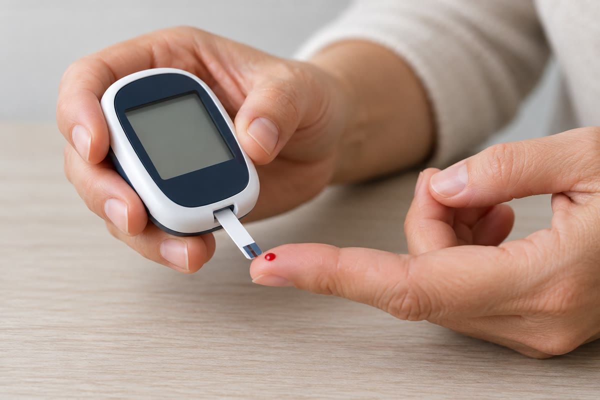
A drop of blood on a strip of plastic, five seconds, a number: the glucose meter that millions of people use several times a day is an electrochemical cell, and what it measures is not a voltage but a current. An enzyme oxidises the glucose, a dissolved iron complex carries the electrons to a carbon electrode, and the current that flows is set by how fast that complex diffuses to the electrode, hence by its concentration. This chapter explains why electrons cross an interface fast or slowly (the Butler–Volmer equation), how mass transport limits the current, and how cyclic voltammetry and the other electroanalytical methods turn currents into concentrations, rate constants and mechanisms.

You already know

The Year 1 volume defined the electrode potential, the standard potential, the Nernst equation, reference electrodes and half-cells. The Year 2 volume introduced current–potential curves with their anodic and cathodic currents, working and counter electrodes, overpotentials, fast and slow systems, the diffusion layer and the limiting current; activity coefficients and ionic strength; calibration curves, the standard-addition method and the limit of detection. Chapter 12 gave transition-state theory. From physics: Fick’s laws of diffusion, Poisson’s equation and capacitors.

A blood-glucose meter: the strip carries a tiny three-electrode cell with an enzyme and a redox mediator; the meter applies a potential and reads a current.

15.1 The electrode–solution interface

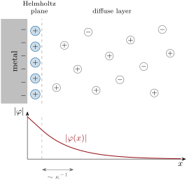
A metal plunged into an electrolyte solution carries a surface charge, and the solution answers with an equal and opposite charge made of an excess of ions of one sign. The two layers of charge form a capacitor of molecular thickness.

Definition 15.1 (Electrical double layer)

The electrical double layer is the arrangement of charge at an electrode–solution interface: the charge on the metal and the compensating ionic charge in the solution. Its compact part, the Helmholtz layer, is the layer of ions and solvent molecules in contact with the surface; its diffuse layer is the region beyond, where thermal motion spreads the excess ions over a distance of the order of the Debye length $\kappa^{-1}$ . The double-layer capacitance $C_{\mathrm{dl}}$ is the charge stored per unit area per volt of potential across the interface.

Proposition 15.2 (Debye length)

In a solution of ionic strength $I$ (in $\mathrm{mol}\,\mathrm{m}^{-3}$ ) and relative permittivity $\varepsilon_r$ , a small potential $\varphi_0$ at the electrode decays into the solution as $\varphi = \varphi_0\eu^{-\kappa x}$ , with

\kappa^{-1} = \sqrt{\frac{\varepsilon_r\varepsilon_0RT}{2F^2I}} .

Proof. Poisson’s equation (from physics) relates the potential to the charge density: $\dd^2\varphi/\dd x^2 = -\rho/\varepsilon_r\varepsilon_0$ . Each ion obeys the Boltzmann distribution in the potential: $c_i = c_i^{\circ}\eu^{-z_iF\varphi/RT}$ , so $\rho = F\sum_iz_ic_i^{\circ}\eu^{-z_iF\varphi/RT}$ . For $F\varphi \ll RT$ , $\eu^{-z_iF\varphi/RT} \approx 1 - z_iF\varphi/RT$ ; the zero-order terms cancel by electroneutrality, and $\rho \approx -(F^2/RT)\sum_iz_i^2c_i^{\circ}\,\varphi = -(2F^2I/RT)\varphi$ . Hence $\dd^2\varphi/\dd x^2 = \kappa^2\varphi$ , whose solution vanishing far away is $\varphi_0\eu^{-\kappa x}$ . ∎

Example 15.3 (The thickness of the double layer)

In water at $298.15\,\mathrm{K}$ ( $\varepsilon_r = 78.4$ ) with $0.10\,\mathrm{mol}/\mathrm{L}$ of a 1:1 salt ( $I = 100\,\mathrm{mol}\,\mathrm{m}^{-3}$ ), $\kappa^{-1} = \sqrt{78.4 \times 8.854 \times 10^{-12} \times 2479/(2 \times 96\,485^2 \times 100)} = 0.96\,\mathrm{nm}$ ; at $1.0\,\mathrm{mmol}/\mathrm{L}$ , ten times more. A supporting electrolyte compresses the diffuse layer to a few molecular diameters.

The diffuse layer behaves as a capacitor whose plates are $\kappa^{-1}$ apart: its capacitance per unit area at low potential is $\varepsilon_r\varepsilon_0\kappa$ (the Gouy–Chapman result; its dependence on the potential is admitted). In series with the compact Helmholtz layer, it gives the measured $C_{\mathrm{dl}}$ , of the order of tens of microfarads per square centimetre (the Stern model). Whenever the potential changes, this capacitor charges: a scan at $v$ volts per second draws a charging current $C_{\mathrm{dl}}Av$ that carries no chemistry and adds to every voltammetric measurement.

The electrical double layer (Gouy–Chapman–Stern model, schematic): a negatively charged metal, a compact layer of cations at the Helmholtz plane, and a diffuse layer where cations outnumber anions over a few Debye lengths. Below, the size of the potential (negative, like the charge of the metal) falls linearly across the compact layer, then exponentially in the diffuse layer.

15.2 Electron-transfer kinetics

Consider the reduction $\mathrm{O} + n\,\mathrm{e}^- \to \mathrm{R}$ at an electrode held at the potential $E$ , whose equilibrium potential for the bulk solution would be $E_{\mathrm{eq}}$ . The overpotential is $\eta = E - E_{\mathrm{eq}}$ .

Definition 15.4 (Exchange current density, transfer coefficient, standard rate constant)

At equilibrium the anodic and cathodic currents are equal and opposite; their common magnitude per unit area is the exchange current density $j_0$ . The transfer coefficient $\alpha$ ( $0 < \alpha < 1$ ) is the fraction of the electrical energy $nF\eta$ that lowers the barrier of the cathodic reaction. The standard rate constant $k^\circ$ is the common value of the cathodic and anodic rate constants at the formal potential $E^{\circ\prime}$ .

Theorem 15.5 (Butler–Volmer equation)

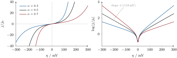
If the surface concentrations equal the bulk ones (no mass-transport limitation), the current density at overpotential $\eta$ is, counting anodic currents positive,

j = j_0\bigl[\eu^{(1 - \alpha)f\eta} - \eu^{-\alpha f\eta}\bigr], \qquad f = \frac{nF}{RT}.

This is the Butler–Volmer equation.

Proof. By transition-state theory the cathodic and anodic rate constants are $k_{\mathrm c} = A\eu^{-\Delta G_{\mathrm c}^{\ddagger}/RT}$ and $k_{\mathrm a} = A\eu^{-\Delta G_{\mathrm a}^{\ddagger}/RT}$ . Changing the electrode potential by $\delta E$ changes the Gibbs energy of the reaction $\mathrm{O} + n\,\mathrm{e}^- \to \mathrm{R}$ by $nF\,\delta E$ (the electrons in the metal gain $-nF\,\delta E$ of electrical energy). Assume, to first order, that a fraction $\alpha$ of this change goes into the cathodic barrier and the rest into the anodic one: $\Delta G_{\mathrm c}^{\ddagger} \to \Delta G_{\mathrm c}^{\ddagger} + \alpha nF\,\delta E$ , $\Delta G_{\mathrm a}^{\ddagger} \to \Delta G_{\mathrm a}^{\ddagger} - (1 - \alpha)nF\,\delta E$ . Measuring $\delta E$ from the equilibrium potential, where the two currents are both $j_0$ in magnitude, gives $j_{\mathrm c} = j_0\eu^{-\alpha f\eta}$ and $j_{\mathrm a} = j_0\eu^{(1 - \alpha)f\eta}$ ; the net current is their difference. ∎

Corollary 15.6 (Charge-transfer resistance)

For $|\eta| \ll RT/nF$ , $j = j_0f\eta$ : the interface behaves as a resistance $R_{\mathrm{ct}} = RT/(nFi_0)$ , with $i_0 = j_0A$ .

Proof. Expand both exponentials to first order: $j = j_0[(1 - \alpha)f\eta + \alpha f\eta] = j_0f\eta$ ; then $\eta/i = 1/(fi_0)$ . ∎

Corollary 15.7 (Tafel equation)

For $\eta \ll -RT/nF$ (a strongly cathodic overpotential), the anodic term is negligible and

\eta = \frac{2.303\,RT}{\alpha nF}\bigl(\log j_0 - \log|j|\bigr):

$\log|j|$ is linear in $\eta$ , with a slope of $1/(\text{$118\,\mathrm{mV}$})$ per decade at $298\,\mathrm{K}$ for $\alpha = 0.5$ , $n = 1$ . This is the Tafel equation.

Proof. $|j| = j_0\eu^{-\alpha f\eta}$ , so $\ln|j| = \ln j_0 - \alpha f\eta$ ; convert to decimal logarithms. ∎

Definition 15.8 (Charge-transfer resistance, Tafel slope)

The charge-transfer resistance of an electrode is $R_{\mathrm{ct}} = (\partial\eta/\partial i)_{\eta = 0}$ . The Tafel slope is the change of overpotential per decade of current in the Tafel region, $2.303\,RT/\alpha nF$ .

The Butler–Volmer equation (n = 1, 298\, K) for three transfer coefficients. Left: the current is linear in near equilibrium (the charge-transfer resistance) and exponential beyond; makes it asymmetric. Right: the Tafel plot, whose straight branches extrapolate to |j/j_0| = 0 at = 0; the dashed line is the cathodic Tafel line for = 0.5. — The Butler–Volmer equation ( $n = 1$ , $298\,\mathrm{K}$ ) for three transfer coefficients. Left: the current is linear in $\eta$ near equilibrium (the charge-transfer resistance) and exponential beyond; $\alpha$ makes it asymmetric. Right: the Tafel plot, whose straight branches extrapolate to $\log|j/j_0| = 0$ at $\eta = 0$ ; the dashed line is the cathodic Tafel line for $\alpha = 0.5$ .

Method 15.9 (A Tafel analysis)

Record the steady current against $\eta$ in a stirred solution, well below the limiting current (or correct for mass transport).
Plot $\log|i|$ against $\eta$ ; fit the linear branch beyond about $100\,\mathrm{mV}$ .
The slope gives $\alpha$ (or $1 - \alpha$ on the anodic branch); the intercept at $\eta = 0$ gives $\log i_0$ .
Check: near $\eta = 0$ , the slope of $i$ against $\eta$ is $1/R_{\mathrm{ct}} = nFi_0/RT$ .

The fast and slow systems of the Year 2 volume are the two ends of this picture: a fast system has a large $j_0$ and its current–potential curve rises steeply at the equilibrium potential; a slow system needs a large overpotential before any current flows. The exchange current density of the same reaction varies over many orders of magnitude from one electrode material to another: hydrogen evolution is fast on platinum and extremely slow on mercury.

15.3 Mass transport

Definition 15.10 (Modes of mass transport)

Species reach an electrode by migration, the motion of ions in the electric field; by diffusion, down concentration gradients; and by convection, the motion of the solution as a whole (stirring, rotation, flow). A supporting electrolyte is an inert salt added in large excess, which carries almost all the current through the solution, so that the electroactive species moves by diffusion and convection only.

Definition 15.11 (Chronoamperometry)

Chronoamperometry records the current against time after a step of the electrode potential.

Theorem 15.12 (Cottrell equation)

After a potential step at $t = 0$ to a value where the electroactive species is consumed as soon as it reaches a planar electrode of area $A$ , in a quiet solution with a supporting electrolyte, the current is

i = nFAc^*\sqrt{\frac{D}{\pi t}},

where $c^*$ is the bulk concentration and $D$ the diffusion coefficient. This is the Cottrell equation.

Proof. The concentration obeys Fick’s second law $\partial c/\partial t = D\,\partial^2c/\partial x^2$ , with $c(x, 0) = c^*$ , $c(0, t) = 0$ for $t > 0$ and $c \to c^*$ far away. The function $c = c^*\operatorname{erf}(x/2\sqrt{Dt})$ , with $\operatorname{erf}u = \frac{2}{\sqrt\pi}\int_0^u\eu^{-s^2}\dd s$ , satisfies these conditions: $\operatorname{erf}0 = 0$ , $\operatorname{erf}u \to 1$ as $u \to \infty$ (at $t \to 0$ for every $x > 0$ , and far away). With $u = x/2\sqrt{Dt}$ , $\partial c/\partial t = c^*\frac{2}{\sqrt\pi}\eu^{-u^2}\partial u/\partial t = -c^*\frac{2}{\sqrt\pi}\eu^{-u^2}\frac{u}{2t}$ and $\partial^2c/\partial x^2 = c^*\frac{2}{\sqrt\pi}(-2u)\eu^{-u^2}\frac{1}{4Dt}$ : the two sides of Fick’s law agree. The current is the flux at the surface: $i = nFAD(\partial c/\partial x)_{x = 0} = nFADc^*\frac{2}{\sqrt\pi}\frac{1}{2\sqrt{Dt}} = nFAc^*\sqrt{D/\pi t}$ . (Uniqueness of the solution is admitted.) ∎

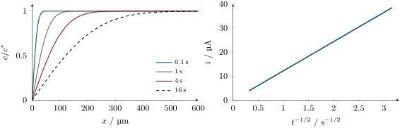
Chronoamperometry (model: D = 1.0 × 10-5\, cm2\, s-1, c* = 1.0\, mM, a 3\, mm disk). Left: the depletion layer grows as √Dt, about 30\, µ m after 0.1\, s and 350\, µ m after 16\, s. Right: the Cottrell current is proportional to t-1/2; its slope gives D. — Chronoamperometry (model: $D = 1.0 \times 10^{-5}\,\mathrm{cm}^{2}\,\mathrm{s}^{-1}$ , $c^* = 1.0\,\mathrm{mM}$ , a $3\,\mathrm{mm}$ disk). Left: the depletion layer grows as $\sqrt{Dt}$ , about $30\,\text{µ}\mathrm{m}$ after $0.1\,\mathrm{s}$ and $350\,\text{µ}\mathrm{m}$ after $16\,\mathrm{s}$ . Right: the Cottrell current is proportional to $t^{-1/2}$ ; its slope gives $D$ .

A stirred solution or a rotating disk electrode holds the diffusion layer at a constant thickness $\delta$ : the current reaches the steady limiting value $nFADc^*/\delta$ of the Year 2 volume. For a rotating disk, $\delta$ decreases as the inverse square root of the rotation rate (Levich, admitted), which makes the limiting current proportional to $\sqrt\omega$ .

15.4 Cyclic voltammetry

Definition 15.13 (Cyclic voltammetry)

Cyclic voltammetry sweeps the potential of a stationary working electrode linearly with time between two limits and back, at a scan rate $v$ , in a quiet solution, and records the current. The plot of current against potential is the voltammogram; each wave has a peak current $i_{\mathrm p}$ at its peak potential $E_{\mathrm p}$ .

The peak arises from two competing effects. As the potential moves past $E^{\circ\prime}$ , the surface concentration of the reactant falls (the Nernst equation, for a fast system) and the current grows; but the depleted layer thickens with time and the flux falls. On the return sweep the product, still near the electrode, is converted back.

Definition 15.14 (Reversibility)

With the dimensionless rate parameter $\Lambda = k^\circ/\sqrt{DnFv/RT}$ , comparing the electron-transfer rate with the rate of diffusion imposed by the scan, a couple is electrochemically reversible if $\Lambda > 15$ (its surface concentrations obey the Nernst equation at all times), quasi-reversible if $15 > \Lambda > 10^{-2(1 + \alpha)}$ , and electrochemically irreversible below.

Remark 15.15

The fast and slow systems of the Year 2 volume correspond to this classification, but with a difference: reversibility here depends on the scan rate. The same couple can be reversible at $10\,\mathrm{mV}/\mathrm{s}$ and quasi-reversible at $10\,\mathrm{V}/\mathrm{s}$ , since a faster scan leaves less time for electron transfer.

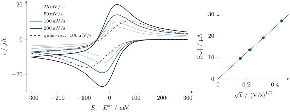
Proposition 15.16 (Randles–Ševčík equation)

For a reversible wave on a planar electrode at $298\,\mathrm{K}$ ,

i_{\mathrm p} = 0.4463\,nFAc^*\sqrt{\frac{nFvD}{RT}},

so that $i_{\mathrm p} \propto \sqrt v$ . This is the Randles–Ševčík equation.

Partial proof. In the variables $\xi = x\sqrt{nFv/(RTD)}$ and $\theta = nFvt/RT$ (the potential sweep in units of $RT/nF$ ), Fick’s law with the Nernst condition at the surface contains no parameter other than the starting potential: the dimensionless flux is a universal function $\chi(\theta)$ . Back in physical units, $i = nFAc^*\sqrt{nFvD/RT}\,\chi(\theta)$ : every current, the peak included, scales as $\sqrt v$ . The value 0.4463 of the maximum of $\chi$ comes from a numerical solution (admitted; the simulation of the figure reproduces it to 0.1 %). ∎

Proposition 15.17 (Peak separation)

For a reversible wave, the cathodic and anodic peaks lie about $28.5\,\mathrm{mV}$ $/n$ on either side of $E^{\circ\prime}$ (at $298\,\mathrm{K}$ , for a switching potential far beyond the wave): $\Delta E_{\mathrm p} \approx 57/n$ mV, independent of the scan rate, and $E_{1/2} = (E_{\mathrm{pc}} + E_{\mathrm{pa}})/2 = E^{\circ\prime}$ when the two species have equal diffusion coefficients.

Partial proof. In the dimensionless form of the previous proof, the peak occurs at a fixed value of $\theta$ , that is at a fixed potential relative to $E^{\circ\prime}$ , whatever $v$ ; the symmetry of the Nernst condition between O and R places the anodic peak symmetrically. The numerical value is admitted; the simulation gives $\pm28.5\,\mathrm{mV}$ , $\Delta E_{\mathrm p} = 57.7\,\mathrm{mV}$ . ∎

Cyclic voltammograms simulated by finite differences for a reduction (model: 1.0\, mM, D = 1.0 × 10-5\, cm2\, s-1, 3\, mm disk, n = 1; anodic current positive). Reversible waves at four scan rates: the peaks stay 57.7\, mV apart, centred on E, and the peak current grows as √ v (right, the line is the Randles–Ševčík equation). Dashed: a quasi-reversible couple (k = 2 × 10-3\, cm\, s-1) at 100\, mV/ s, with peaks 162\, mV apart and lower. — Cyclic voltammograms simulated by finite differences for a reduction (model: $1.0\,\mathrm{mM}$ , $D = 1.0 \times 10^{-5}\,\mathrm{cm}^{2}\,\mathrm{s}^{-1}$ , $3\,\mathrm{mm}$ disk, $n = 1$ ; anodic current positive). Reversible waves at four scan rates: the peaks stay $57.7\,\mathrm{mV}$ apart, centred on $E^{\circ\prime}$ , and the peak current grows as $\sqrt v$ (right, the line is the Randles–Ševčík equation). Dashed: a quasi-reversible couple ( $k^\circ = 2 \times 10^{-3}\,\mathrm{cm}\,\mathrm{s}^{-1}$ ) at $100\,\mathrm{mV}/\mathrm{s}$ , with peaks $162\,\mathrm{mV}$ apart and lower.

Method 15.18 (Diagnosing a voltammogram)

Reversible: $\Delta E_{\mathrm p} \approx 57/n$ mV at every scan rate, $|i_{\mathrm{pa}}/i_{\mathrm{pc}}| = 1$ , $i_{\mathrm p} \propto \sqrt v$ ; $E_{1/2}$ gives $E^{\circ\prime}$ .
Quasi-reversible: $\Delta E_{\mathrm p}$ grows with the scan rate; its value gives $k^\circ$ .
Irreversible: no return peak; the peak potential shifts by $30/\alpha n$ mV per decade of scan rate.
A following chemical step (EC mechanism): the return peak is smaller than the forward one at slow scans and recovers at fast scans, which outrun the chemistry.
Adsorbed species: $i_{\mathrm p} \propto v$ , not $\sqrt v$ .

Potentials in non-aqueous solvents, where reference electrodes drift, are referred to an internal standard added at the end of the experiment: the ferrocenium/ferrocene couple, fast and well behaved in most organic solvents.

Method 15.19 (Setting up a three-electrode measurement)

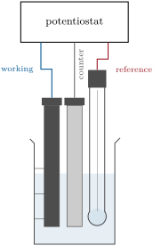
Working electrode (glassy carbon, platinum, gold) freshly polished; counter electrode (platinum wire) of larger area; reference electrode (Ag/AgCl, or a silver wire with an internal standard) near the working electrode.
Solution of the analyte (about 1 mM) with $0.1\,\mathrm{mol}/\mathrm{L}$ of supporting electrolyte, degassed with argon (dissolved oxygen is reduced at moderately negative potentials and would add its own waves).
The potentiostat holds the potential between working and reference electrodes and passes the current between working and counter electrodes; no current flows through the reference.

A three-electrode cell. The potentiostat controls the potential of the working electrode against the reference electrode, which carries no current, and drives the current through the counter electrode.

15.5 Electroanalytical methods

Definition 15.20 (Amperometry, biosensor)

Amperometry measures the current at a fixed potential, proportional to the concentration of the species that reacts. A biosensor couples a biological recognition element (an enzyme, an antibody) to a transducer, here an electrode.

In the glucose strip, glucose oxidase oxidises glucose to gluconolactone and is regenerated by a mediator, hexacyanoferrate(III), which is reduced; at the electrode, held at a potential where hexacyanoferrate(II) is oxidised, the current measures the mediator formed, two per glucose:

\ce{C6H12O6 + 2 [Fe(CN)6]^3- -> C6H10O6 + 2 [Fe(CN)6]^4- + 2 H+} .

Definition 15.21 (Anodic stripping voltammetry)

Anodic stripping voltammetry preconcentrates a metal by reducing its ions onto an electrode for a fixed time at a fixed potential, then scans the potential anodically and measures the current peak of its re-oxidation, which is proportional to the concentration in the solution.

The preconcentration makes the method sensitive enough for traces of lead or cadmium in drinking water, at the level of micrograms per litre. Since the sensitivity depends on the matrix, it is calibrated in the sample itself, by standard additions.

Method 15.22 (Standard additions with stripping)

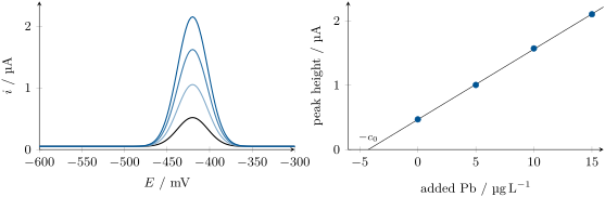
Record the stripping peak of the sample, then after three or more additions of a standard, each raising the concentration by a known amount (small volumes, so that dilution is negligible or corrected).
Fit the peak height against the added concentration: a straight line.
Its intercept on the concentration axis is minus the concentration of the sample; propagate the standard errors of the line to the result.

Anodic stripping of lead with three standard additions (data of ). Left: the stripping peaks grow with each addition. Right: the least-squares line of peak height against added concentration crosses the axis at minus the concentration of the sample. — Anodic stripping of lead with three standard additions (data of Exercise 15.9). Left: the stripping peaks grow with each addition. Right: the least-squares line of peak height against added concentration crosses the axis at minus the concentration of the sample.

Definition 15.23 (Ion-selective electrode, selectivity coefficient)

An ion-selective electrode is an electrode whose potential, through a membrane that exchanges one ion preferentially, depends on the activity of that ion. Its selectivity coefficient $K_{ij}$ measures its response to an interfering ion $j$ relative to the primary ion $i$ .

Proposition 15.24 (Nikolsky equation)

For a primary ion $i$ of charge $z_i$ and an interfering ion $j$ of charge $z_j$ ,

E = \text{const} + \frac{RT}{z_iF}\ln\bigl(a_i + K_{ij}a_j^{z_i/z_j}\bigr) .

This is the Nikolsky equation.

Partial proof. For a membrane permeable to $i$ only, the equality of electrochemical potentials across it gives a Nernst-type potential, $\frac{RT}{z_iF}\ln a_i$ plus a constant. If $j$ can replace $i$ in the membrane by ion exchange, with an exchange constant that defines $K_{ij}$ , the activity of $i$ at the membrane surface is raised by $K_{ij}a_j^{z_i/z_j}$ (the power keeps the charges balanced in the exchange). The detailed derivation is admitted. ∎

The glass pH electrode is the oldest ion-selective electrode; its sodium error, at high pH and high sodium concentration, is the Nikolsky term.

Definition 15.25 (Coulometry)

Coulometry determines the amount of a substance from the total charge passed in its complete electrolysis: $Q = nFn_{\text{substance}}$ (Faraday’s law), with no calibration.

Proposition 15.26 (Uncertainty of a concentration read from a calibration line)

For a calibration line $y = a + bx$ fitted to $n$ standards (residual standard deviation $s$ , mean $\bar y$ , $S_{xx} = \sum(x_i - \bar x)^2$ ), the concentration of a sample whose mean response over $m$ replicates is $y_0$ is $x_0 = (y_0 - a)/b$ , with the standard uncertainty

u(x_0) = \frac{s}{b}\sqrt{\frac1m + \frac1n + \frac{(y_0 - \bar y)^2}{b^2S_{xx}}} .

Proof. Write $x_0 = \bar x + (y_0 - \bar y)/b$ . To first order its variance is $(\operatorname{var}y_0 + \operatorname{var}\bar y)/b^2 + (y_0 - \bar y)^2\operatorname{var}b/b^4$ , the three terms being uncorrelated ( $\bar y$ and $b$ are uncorrelated, Proposition 12.9). With $\operatorname{var}y_0 = s^2/m$ , $\operatorname{var}\bar y = s^2/n$ and $\operatorname{var}b = s^2/S_{xx}$ , the result follows. ∎

The uncertainty is smallest in the middle of the calibration range and grows towards its ends; replicate readings of the sample shrink only the first term.

In the lab — Preparing a glassy-carbon electrode

The electrode is polished on a felt pad with an alumina slurry in a figure-of-eight motion, rinsed, sonicated briefly in water and rinsed again. A voltammogram of a known couple (hexacyanoferrate, ferrocene) checks that the peak separation is close to the reversible value: a larger one signals a fouled surface or an uncompensated resistance. The solution is degassed with argon for ten minutes and kept under a blanket of argon during the scans.

Safety

Lead nitrate, used for the lead standards: oxidiser, may damage fertility and the unborn child, suspected carcinogen, very toxic to aquatic life; standard solutions are bought ready-made and handled with gloves, and all lead waste is collected. Potassium hexacyanoferrate(III): harmful and suspected of damaging fertility; never acidified strongly or heated (it could release hydrogen cyanide). Mercury electrodes, once common in stripping analysis, have been replaced by bismuth-film and carbon electrodes.

History — Heyrovský’s polarograph, 1922

Jaroslav Heyrovský measured in 1922 the current through a mercury electrode that dripped from a fine capillary, renewing its surface every few seconds, against the applied potential. Each reducible species gave a wave whose position identified it and whose height measured its concentration; with Masuzo Shikata he built in 1924 the polarograph, which recorded the curves automatically on photographic paper. Polarography was the first instrumental method of chemical analysis in routine use, and earned Heyrovský the 1959 Nobel Prize in Chemistry.

15.6 Exercises

Exercise 15.1 ★

A Tafel plot of a reduction ( $n = 1$ , $298\,\mathrm{K}$ ) has a cathodic slope of $-118\,\mathrm{mV}$ per decade and extrapolates at $\eta = 0$ to $|j| = 2.0 \times 10^{-6}\,\mathrm{A}\,\mathrm{cm}^{-2}$ (data of the exercise). Give $\alpha$ and $j_0$ .

Solution

Solution of Exercise 15.1.

Cathodic slope $2.303RT/\alpha F = 118\,\mathrm{mV}$ gives $\alpha = 59.2/118 = 0.50$ ; $j_0 = 2.0 \times 10^{-6}\,\mathrm{A}\,\mathrm{cm}^{-2}$ , the intercept at $\eta = 0$ .

Exercise 15.2 ★

An electrode of $0.20\,\mathrm{cm}^{2}$ has $j_0 = 1.0 \times 10^{-3}\,\mathrm{A}\,\mathrm{cm}^{-2}$ for a one-electron couple. Compute its charge-transfer resistance at $298\,\mathrm{K}$ .

Solution

Solution of Exercise 15.2.

$i_0 = 2.0 \times 10^{-4}\,\mathrm{A}$ ; $R_{\mathrm{ct}} = RT/(Fi_0) = 0.02569/2.0 \times 10^{-4} = 128\,\Omega$ .

Exercise 15.3 ★

Compute the Debye length in water at $298.15\,\mathrm{K}$ for $1.0\,\mathrm{mmol}/\mathrm{L}$ and for $0.10\,\mathrm{mol}/\mathrm{L}$ of $\ce{MgSO4}$ .

Solution

Solution of Exercise 15.3.

For $\ce{MgSO4}$ , $I = \frac12(4c + 4c) = 4c$ . At $1.0\,\mathrm{mmol}/\mathrm{L}$ , $I = 4.0\,\mathrm{mol}\,\mathrm{m}^{-3}$ and $\kappa^{-1} = 0.96\,\mathrm{nm} \times \sqrt{100/4} = 4.8\,\mathrm{nm}$ ; at $0.10\,\mathrm{mol}/\mathrm{L}$ , $I = 400\,\mathrm{mol}\,\mathrm{m}^{-3}$ , $\kappa^{-1} = 0.48\,\mathrm{nm}$ .

Exercise 15.4 ★

A cyclic voltammogram at $100\,\mathrm{mV}/\mathrm{s}$ on a $0.0707\,\mathrm{cm}^{2}$ electrode with $C_{\mathrm{dl}} = 20\,\text{µ}\mathrm{F}\,\mathrm{cm}^{-2}$ : compute the charging current, and compare with the $19\,\text{µ}\mathrm{A}$ faradaic peak of the figure. What happens at $10\,\mathrm{V}/\mathrm{s}$ ?

Solution

Solution of Exercise 15.4.

$i_{\mathrm c} = C_{\mathrm{dl}}Av = 20 \times 10^{-6} \times 0.0707 \times 0.1 = 0.14\,\text{µ}\mathrm{A}$ , under 1 % of the peak. At $10\,\mathrm{V}/\mathrm{s}$ it is $14\,\text{µ}\mathrm{A}$ , while the peak grows only to $19\sqrt{100} = 190\,\text{µ}\mathrm{A}$ : the charging current grows as $v$ , the faradaic one as $\sqrt v$ .

Exercise 15.5 ★★

After a potential step, $i\sqrt t = 12.2\,\text{µ}\mathrm{A}\,\mathrm{s}^{1/2}$ for a one-electron reduction of a $1.00\,\mathrm{mM}$ solution at a $0.0707\,\mathrm{cm}^{2}$ electrode. Compute $D$ .

Solution

Solution of Exercise 15.5.

$D = \pi\bigl(i\sqrt t/nFAc^*\bigr)^2 = \pi(12.2 \times 10^{-6}/(96\,485 \times 0.0707 \times 1.00 \times 10^{-6}))^2 = 1.0 \times 10^{-5}\,\mathrm{cm}^{2}\,\mathrm{s}^{-1}$ .

Exercise 15.6 ★★

Compute the Randles–Ševčík peak current for $n = 1$ , $A = 0.0707\,\mathrm{cm}^{2}$ , $c^* = 2.0\,\mathrm{mM}$ , $D = 7.0 \times 10^{-6}\,\mathrm{cm}^{2}\,\mathrm{s}^{-1}$ at $50\,\mathrm{mV}/\mathrm{s}$ and at $500\,\mathrm{mV}/\mathrm{s}$ .

Solution

Solution of Exercise 15.6.

$FAc^* = 1.364 \times 10^{-2}\,\mathrm{C}\,\mathrm{cm}^{-1}$ , $F/RT = 38.92\,\mathrm{V}^{-1}$ . At $50\,\mathrm{mV}/\mathrm{s}$ : $\sqrt{38.92 \times 0.05 \times 7.0 \times 10^{-6}} = 3.69 \times 10^{-3}$ , $i_{\mathrm p} = 0.4463 \times 1.364 \times 10^{-2} \times 3.69 \times 10^{-3} = 22.5\,\text{µ}\mathrm{A}$ ; at $500\,\mathrm{mV}/\mathrm{s}$ , $\sqrt{10}$ times more, $71\,\text{µ}\mathrm{A}$ .

Exercise 15.7 ★★

Three couples give, at 50 and $500\,\mathrm{mV}/\mathrm{s}$ : (a) $\Delta E_{\mathrm p} = 58$ and 59 mV, $|i_{\mathrm{pa}}/i_{\mathrm{pc}}| = 1.0$ ; (b) $\Delta E_{\mathrm p} = 75$ and 140 mV, $|i_{\mathrm{pa}}/i_{\mathrm{pc}}| = 1.0$ ; (c) $\Delta E_{\mathrm p}$ undefined at $50\,\mathrm{mV}/\mathrm{s}$ (no return peak), a return peak with $|i_{\mathrm{pa}}/i_{\mathrm{pc}}| = 0.8$ at $500\,\mathrm{mV}/\mathrm{s}$ . Diagnose each.

Solution

Solution of Exercise 15.7.

(a) Reversible. (b) Quasi-reversible: the separation grows with the scan rate. (c) A chemical step follows the electron transfer (EC): at slow scans the product is consumed before the return sweep; a fast scan outruns the chemistry.

Exercise 15.8 ★★

A potassium-selective electrode has $K_{\ce{K+},\ce{Na+}} = 2 \times 10^{-4}$ . In a sample with $a(\ce{K+}) = 4.0 \times 10^{-3}\,$ and $a(\ce{Na+}) = 0.14$ , what is the relative error on the potassium activity if sodium is ignored?

Solution

Solution of Exercise 15.8.

$K_{ij}a_j/a_i = 2 \times 10^{-4} \times 0.14/4.0 \times 10^{-3} = 0.007$ : the electrode reads 0.7 % high.

Exercise 15.9 ★★

Stripping peaks of a water sample with 0, 5, 10 and $15\,\text{µ}\mathrm{g}\,\mathrm{L}^{-1}$ of added lead are 0.468, 1.003, 1.571 and $2.101\,\text{µ}\mathrm{A}$ (data of the exercise). Compute the lead concentration of the measured solution with its standard uncertainty.

Solution

Solution of Exercise 15.9.

Least squares: $b = 0.1093\,\text{µ}\mathrm{A}\,\mathrm{L}\,\text{µ}\mathrm{g}^{-1}$ , $a = 0.466\,\text{µ}\mathrm{A}$ , $s = 0.011\,\text{µ}\mathrm{A}$ ; $c_0 = a/b = 4.26\,\text{µ}\mathrm{g}\,\mathrm{L}^{-1}$ , with $u(c_0) = \frac sb\sqrt{\frac1n + \frac{\bar y^2}{b^2S_{xx}}} = 0.12\,\text{µ}\mathrm{g}\,\mathrm{L}^{-1}$ ( $n = 4$ , $\bar y = 1.286$ , $S_{xx} = 125$ ).

Exercise 15.10 ★★★

A copper coulometer passes a constant $50.0\,\mathrm{mA}$ for $30.0\,\mathrm{min}$ and deposits copper from $\ce{Cu^{2+}}$ . Compute the mass deposited; why does coulometry need no calibration?

Solution

Solution of Exercise 15.10.

$Q = 0.0500 \times 1800 = 90.0\,\mathrm{C}$ ; $n(\ce{Cu}) = Q/2F = 4.66 \times 10^{-4}\,\mathrm{mol}$ , $29.6\,\mathrm{mg}$ . The result depends only on the charge, measured from a current and a time, and on Faraday’s constant: no standard is needed, provided the electrolysis is complete and its current efficiency is 100 %.

Exercise 15.11 ★★★

For a couple with $k^\circ = 1.0 \times 10^{-2}\,\mathrm{cm}\,\mathrm{s}^{-1}$ and $D = 1.0 \times 10^{-5}\,\mathrm{cm}^{2}\,\mathrm{s}^{-1}$ , compute $\Lambda$ at $0.1\,\mathrm{V}/\mathrm{s}$ and $10\,\mathrm{V}/\mathrm{s}$ ( $n = 1$ , $298\,\mathrm{K}$ ) and classify the wave at each scan rate.

Solution

Solution of Exercise 15.11.

$\sqrt{DFv/RT} = \sqrt{1.0 \times 10^{-5} \times 38.92 \times 0.1} = 6.24 \times 10^{-3}\,\mathrm{cm}\,\mathrm{s}^{-1}$ : $\Lambda = 1.6$ , quasi-reversible. At $10\,\mathrm{V}/\mathrm{s}$ , $\Lambda = 0.16$ , still quasi-reversible but further from the reversible limit; the wave would be reversible only below about $1\,\mathrm{mV}/\mathrm{s}$ .

Exercise 15.12 ★★★

A calibration line from $n = 7$ standards has $b = 0.919\,\text{µ}\mathrm{A}\,\mathrm{mM}^{-1}$ , $s = 0.077\,\text{µ}\mathrm{A}$ , $\bar y = 8.89\,\text{µ}\mathrm{A}$ and $S_{xx} = 241\,\mathrm{mM}^{2}$ . Compute the uncertainty of a concentration read from one reading at $y_0 = \bar y$ and at $y_0 = 18.0\,\text{µ}\mathrm{A}$ , and from three readings at $\bar y$ .

Solution

Solution of Exercise 15.12.

$s/b = 0.0838\,\mathrm{mM}$ and $b^2S_{xx} = 203.5\,\text{µ}\mathrm{A}^{2}$ . At $\bar y$ : $0.0838\sqrt{1 + 1/7} = 0.090\,\mathrm{mM}$ . At $18.0\,\text{µ}\mathrm{A}$ : $0.0838\sqrt{1.143 + 83.0/203.5} = 0.104\,\mathrm{mM}$ . Three readings at $\bar y$ : $0.0838\sqrt{1/3 + 1/7} = 0.058\,\mathrm{mM}$ .

15.7 Problem: The Glucose Strip

Problem 15.1

Weekend problem — the glucose strip: the enzyme and its mediator, chronoamperometry and the diffusion coefficient, the calibration line and a blood sample with its uncertainty, and the interference of ascorbate

A test strip carries glucose oxidase, potassium hexacyanoferrate(III) and a carbon working electrode of $0.0300\,\mathrm{cm}^{2}$ . Data of the problem: (a) a strip filled with $10.0\,\mathrm{mM}$ hexacyanoferrate(II) and stepped to an oxidising potential gives the currents 42.0, 29.3, 24.1, 20.8 and $18.7\,\text{µ}\mathrm{A}$ at 1, 2, 3, 4 and $5\,\mathrm{s}$ ; (b) glucose standards of 2.0, 4.0, 6.0, 8.0, 10.0, 15.0 and $20.0\,\mathrm{mM}$ give, at $5.0\,\mathrm{s}$ , 2.16, 4.08, 5.83, 7.78, 9.45, 14.23 and $18.69\,\text{µ}\mathrm{A}$ ; (c) a blood sample gives $7.10\,\text{µ}\mathrm{A}$ .

Part I — The chemistry.

Write the half-reactions of glucose (to gluconolactone, $\ce{C6H10O6}$ ) and of the mediator, and the balanced overall reaction.
How many electrons reach the electrode per glucose molecule?
Why is a mediator used rather than oxygen, the natural partner of the enzyme?
Why is the electrode held at a potential where hexacyanoferrate(II) is oxidised, well beyond its formal potential?
Why must the reading be taken at a fixed time after the drop is applied?

Part II — Chronoamperometry.

Which law should the currents of (a) follow? Check it on the data.
Fit $i$ against $t^{-1/2}$ through the origin: the slope is $41.8\,\text{µ}\mathrm{A}\,\mathrm{s}^{1/2}$ . Deduce $D$ of hexacyanoferrate(II).
Compute the thickness $\sqrt{\pi Dt}$ of the depletion layer after $5\,\mathrm{s}$ . Is the planar model reasonable for a strip whose solution layer is about $100\,\text{µ}\mathrm{m}$ thick?
What would the current be at $5\,\mathrm{s}$ with $5.0\,\mathrm{mM}$ instead of $10.0\,\mathrm{mM}$ ?

Part III — Calibration.

The least-squares line of (b) has $a = 0.356\,\text{µ}\mathrm{A}$ ( $s_a = 0.054$ ), $b = 0.9189\,\text{µ}\mathrm{A}\,\mathrm{mM}^{-1}$ ( $s_b = 0.0049$ ), $s = 0.077\,\text{µ}\mathrm{A}$ . What does $a$ represent?
Is the response linear over the range? What would limit it at high glucose?
Compute the glucose concentration of the blood sample.
With $\bar y = 8.89\,\text{µ}\mathrm{A}$ and $S_{xx} = 241\,\mathrm{mM}^{2}$ , compute its standard uncertainty.
Which term of the uncertainty dominates, and how could it be reduced?
Estimate the limit of detection as $3s/b$ .
Express the result in milligrams per decilitre (molar mass of glucose $180.16\,\mathrm{g}/\mathrm{mol}$ ).

Part IV — Interferents.

Ascorbate (vitamin C) is oxidised directly at the electrode. What does it do to the reading?
How would a cyclic voltammogram of the strip reveal it?
Why does a lower working potential, made possible by a better mediator, reduce such interferences?
A blank electrode without enzyme, read at the same time, gives $0.25\,\text{µ}\mathrm{A}$ more than the calibration intercept with a given sample. How is it used?
How does the temperature of the strip affect the current, through $D$ ?
Why are the standards prepared in a blood-like matrix?
Why is the uncertainty of the meter in practice larger than the one computed in Part III?
State the result: the glucose concentration of the sample with its standard uncertainty.

Solution

Solution of Problem 15.1.

1. $\ce{C6H12O6 -> C6H10O6 + 2 H+ + 2 e-}$ and $\ce{[Fe(CN)6]^3- + e- -> [Fe(CN)6]^4-}$ ; overall

\ce{C6H12O6 + 2 [Fe(CN)6]^3- -> C6H10O6 + 2 [Fe(CN)6]^4- + 2 H+} .

At the electrode, $\ce{[Fe(CN)6]^4- -> [Fe(CN)6]^3- + e-}$ . 2. Two. 3. Dissolved oxygen in blood is low and variable, and its product, hydrogen peroxide, is oxidised only at a high potential where many other species react; the mediator is present in a known excess. 4. So that its surface concentration is zero: the current is then limited by diffusion only and insensitive to small changes of potential. 5. The current falls as $t^{-1/2}$ ; readings must be taken at the time used for the calibration. 6. Cottrell: $i\sqrt t = 42.0$ , 41.4, 41.7, 41.6, 41.8: constant within 1 %. 7. $D = \pi(\text{slope}/FAc)^2 = \pi(41.8 \times 10^{-6}/(96\,485 \times 0.0300 \times 1.00 \times 10^{-5}))^2 = 6.55 \times 10^{-6}\,\mathrm{cm}^{2}\,\mathrm{s}^{-1}$ . 8. $\sqrt{\pi \times 6.55 \times 10^{-6} \times 5} = 0.010\,\mathrm{cm} = 100\,\text{µ}\mathrm{m}$ : the depletion reaches the top of the layer at about $5\,\mathrm{s}$ ; later readings would fall below the Cottrell law. 9. Half: $9.35\,\text{µ}\mathrm{A}$ . 10. The background current: oxidation of interferents and impurities, charging, the mediator’s own residual hexacyanoferrate(II). 11. Yes: the residuals, at most $0.095\,\text{µ}\mathrm{A}$ , scatter without trend. At high glucose the mediator, present in a limited amount, or the enzyme saturates and the line bends. 12. $(7.10 - 0.356)/0.9189 = 7.34\,\mathrm{mM}$ . 13. $0.0838\sqrt{1 + 1/7 + (7.10 - 8.89)^2/203.5} = 0.0838 \times 1.076 = 0.090\,\mathrm{mM}$ . 14. The $1/m$ term (a single reading); repeated readings, or several strips, reduce it. 15. $3 \times 0.077/0.919 = 0.25\,\mathrm{mM}$ . 16. $7.34 \times 180.16 = 1322\,\mathrm{mg}\,\mathrm{L}^{-1} = 132\,\mathrm{mg}\,\mathrm{dL}^{-1}$ . 17. It adds its own oxidation current: the meter reads too high. 18. A voltammogram of the strip without glucose shows an anodic wave of ascorbate where hexacyanoferrate(II) is oxidised. 19. Fewer substances are oxidised at a lower potential. 20. The blank current is subtracted from the enzyme electrode’s reading before the calibration line is applied. 21. $D$ grows by a few per cent per kelvin and the current as $\sqrt D$ : meters measure the temperature and correct for it. 22. Viscosity and the red-cell fraction of blood change $D$ and the current; standards in a similar matrix cancel these effects. 23. Strip-to-strip variations (electrode area, enzyme and mediator loading), temperature and blood composition add to the calibration’s own uncertainty. 24. $c(\text{glucose}) = 7.34 \pm 0.09\,\mathrm{mmol}\,\mathrm{L}^{-1}$ (standard uncertainty), about $132\,\mathrm{mg}\,\mathrm{dL}^{-1}$ .

Terms defined in this chapter

See all 852 terms in the glossary