University Chemistry — Year 3 · Bachelor Year 3

3Computational Chemistry: Hartree–Fock and DFT

The helium hydride ion, $\ce{HeH+}$ , is thought to be the first molecule that formed as the young Universe cooled: a helium atom holding a proton. It was made in a laboratory discharge tube in 1925, but searched for in space for decades without success, until its rotational line was detected in a planetary nebula in 2019. By then its bond length, its vibrational frequencies and the wavelengths of its lines had long been known — from calculation. A computer program that solves, approximately, the Schrödinger equation of the electrons can predict the shape, the energy and the spectrum of a molecule nobody has put in a bottle. This chapter explains how such programs work, from the separation of nuclei and electrons to Hartree–Fock theory and density-functional theory, and what their numbers can and cannot be trusted for.

You already know

Chapter 1 gave the Hamiltonian, the Schrödinger equation and the hydrogen atom; Chapter 2 the Slater determinant and the exchange integral. The Year 2 volume built molecular orbitals as linear combinations of atomic orbitals (LCAO), with overlap, Coulomb and resonance integrals and a secular determinant, and solved the Hückel method; it also used photoelectron spectra to see orbital energies.

A computing cluster: rows of servers on which most quantum-chemical calculations now run, often for hours or days per molecule.

3.1 Born–Oppenheimer and the potential energy surface

A molecule’s Hamiltonian contains the kinetic energies of its nuclei and electrons and all their Coulomb interactions. Nuclei are at least 1836 times heavier than electrons: for the same forces they move far more slowly, and the electrons adjust almost instantly to each position of the nuclei.

Definition 3.1 (Born–Oppenheimer approximation)

In the Born–Oppenheimer approximation, the electronic Schrödinger equation is solved for nuclei held fixed at positions $\mathbf R$ ,

\hat H_{\mathrm{el}}\,\psi_{\mathrm{el}}(\mathbf r;\mathbf R) = E_{\mathrm{el}}(\mathbf R)\,\psi_{\mathrm{el}}(\mathbf r;\mathbf R),

and the nuclei then move in the potential $E_{\mathrm{el}}(\mathbf R) + V_{\mathrm{nn}}(\mathbf R)$ , the electronic energy plus the repulsion of the nuclei.

Definition 3.2 (Potential energy surface, stationary point, geometry optimisation)

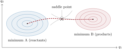
The potential energy surface (PES) of a molecule is the function $U(\mathbf R) = E_{\mathrm{el}}(\mathbf R) + V_{\mathrm{nn}}(\mathbf R)$ of its nuclear coordinates. A stationary point is a point where all first derivatives of $U$ vanish; a minimum is an equilibrium geometry. Searching for one from a starting structure, by following the forces $-\nabla U$ , is a geometry optimisation.

For a diatomic molecule the PES is a curve $U(R)$ ; for a triatomic a function of three coordinates; for $N$ atoms of $3N - 6$ . The mass of the nuclei does not enter $\hat H_{\mathrm{el}}$ : $\ce{H2}$ , $\ce{HD}$ and $\ce{D2}$ share the same PES, the same bond length and force constant, and differ only in how the nuclei move on it (zero-point energy, Chapter 1).

Proposition 3.3 (Frequencies from the Hessian)

Near a minimum, $U \approx U_0 + \frac12\sum_{ij}H_{ij}\,\delta q_i\,\delta q_j$ , with the Hessian $H_{ij} = \partial^2U/\partial q_i\partial q_j$ . In mass-weighted coordinates $\delta q_i\sqrt{m_i}$ , the eigenvalues $\lambda_k$ of the mass-weighted Hessian give the harmonic angular frequencies $\omega_k = \sqrt{\lambda_k}$ of the normal modes. At a minimum all $\lambda_k$ are positive (six, or five for a linear molecule, are zero: translations and rotations); at a first-order saddle point exactly one is negative.

Partial proof. For a diatomic, $U \approx U_0 + \frac12k(R - R_e)^2$ with $k = U''(R_e)$ , and the oscillator of Chapter 1 gives $\omega = \sqrt{k/\mu}$ . In general, the classical equations $m_i\ddot q_i = -\sum_jH_{ij}q_j$ become, in mass-weighted coordinates $x_i = \sqrt{m_i}q_i$ , $\ddot{\mathbf x} = -\tilde H\mathbf x$ with the symmetric matrix $\tilde H_{ij} = H_{ij}/\sqrt{m_im_j}$ ; its eigenvectors oscillate independently at $\sqrt{\lambda_k}$ . A negative $\lambda_k$ gives an imaginary frequency: along that direction the energy goes down, a maximum. The normal modes of Chapter 5 are these eigenvectors. ∎

A potential energy surface seen from above, as a contour map over two nuclear coordinates (schematic). Two minima are joined, through a saddle point (cross), by the path of lowest energy (dashed): the minimum energy path studied in . — A potential energy surface seen from above, as a contour map over two nuclear coordinates (schematic). Two minima are joined, through a saddle point (cross), by the path of lowest energy (dashed): the minimum energy path studied in Chapter 12.

3.2 The variational principle

The electronic Schrödinger equation cannot be solved exactly for any molecule with more than one electron. Approximations are judged by one theorem.

Theorem 3.4 (The variational principle)

For any normalisable trial function $\phi$ satisfying the boundary conditions of the problem,

E[\phi] = \frac{\langle\phi|\hat H|\phi\rangle}{\langle\phi|\phi\rangle} \ge E_0,

where $E_0$ is the lowest eigenvalue of $\hat H$ ; equality holds only if $\phi$ is a ground-state eigenfunction. This is the variational principle.

The lower the energy of a trial function, the better it is; any adjustable parameter is fixed by minimising $E$ .

Proposition 3.5 (Helium with a screened charge)

For helium, the trial function $\phi = \eu^{-\zeta(r_1 + r_2)}$ (in atomic units: lengths in $a_0$ , energies in $E_h$ ) gives $E(\zeta) = \zeta^2 - \frac{27}{8}\zeta$ , minimal for $\zeta = \frac{27}{16}$ , with $E = -(\frac{27}{16})^2 E_h = -2.8477\,E_\mathrm{h}$ .

Proof. For one electron in $\eu^{-\zeta r}$ , $\langle T\rangle = \zeta^2/2$ and $\langle 1/r\rangle = \zeta$ ; the repulsion of two electrons in the same $1s$ function is $\frac58\zeta$ (a standard integral, admitted). So $E = 2\cdot\frac12 \zeta^2 - 2\cdot2\zeta + \frac58\zeta = \zeta^2 - \frac{27}{8}\zeta$ , and $\dd E/\dd \zeta = 0$ gives $\zeta = 27/16 = 1.6875$ . ∎

Example 3.6 (How good is it?)

The total energy of helium is minus the sum of its two ionisation energies, $-(24.5874 + 54.4178)\,\mathrm{eV} = -2.9034\,E_\mathrm{h}$ . The one-parameter function is $0.056\,E_\mathrm{h}$ ( $1.5\,\mathrm{eV}$ ) too high: each electron sees a nucleus screened to $Z_{\mathrm{eff}} = 1.69$ by the other, as Slater’s rules suggest, but the electrons also dodge each other in a way no product of two functions can describe.

Proposition 3.7 (Linear variation)

For a trial function $\phi = \sum_{i=1}^n c_i\chi_i$ built on $n$ fixed functions, with $H_{ij} = \langle\chi_i|\hat H|\chi_j\rangle$ and $S_{ij} = \langle\chi_i|\chi_j \rangle$ , the stationary values of $E$ are the roots of $\det(H - ES) = 0$ , and the lowest root is an upper bound to $E_0$ .

Proof. $E\sum_{ij}c_ic_jS_{ij} = \sum_{ij}c_ic_jH_{ij}$ (real coefficients). Differentiate with respect to $c_k$ and set $\partial E/\partial c_k = 0$ : $\sum_j(H_{kj} - ES_{kj})c_j = 0$ for every $k$ . A non-zero solution needs a vanishing determinant. The lowest root is $E[\phi]$ for its eigenvector, hence $\ge E_0$ . ∎

The Hückel method of the Year 2 volume is this proposition with $p$ orbitals and empirical $H_{ij}$ . Every method below is the same idea with better functions and better matrix elements.

3.3 Basis sets

Definition 3.8 (Basis set, minimal basis, Slater- and Gaussian-type orbitals)

A basis set is the set of fixed functions $\chi_i$ , centred on the atoms, from which molecular orbitals are built. A minimal basis set has one function per occupied atomic orbital (one $1s$ for H, five for C). A Slater-type orbital (STO) has the radial form $r^{n-1}\eu^{-\zeta r}$ ; a Gaussian-type orbital (GTO) has the form $\eu^{-\alpha r^2}$ times a polynomial in $x$ , $y$ , $z$ . A contracted Gaussian function is a fixed combination $\sum_kd_k\,\eu^{-\alpha_kr^2}$ of primitive Gaussians.

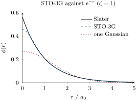
Slater functions have the right shape (a cusp at the nucleus, an exponential tail) but their two-electron integrals over several centres are very costly; Gaussian functions have the wrong shape, but the product of two Gaussians on different centres is a Gaussian on a point between them, so every integral reduces to a closed formula. Contractions get the best of both: in the STO-3G basis, each Slater function is replaced by a fixed sum of three Gaussians fitted to it.

Example 3.9 (The STO-3G function of hydrogen)

The hydrogen $1s$ function of STO-3G is $0.15433\,g(3.42525) + 0.53533\, g(0.62391) + 0.44463\,g(0.16886)$ , where $g(\alpha)$ is the normalised Gaussian $(2\alpha/\pi)^{3/4}\eu^{-\alpha r^2}$ (exponents in $a_0^{-2}$ ). It imitates a Slater function of exponent $\zeta = 1.24$ — a hydrogen atom slightly compressed, as it is in molecules. Its overlap with the exact $1s$ function of the same exponent is $0.9998$ ; only the cusp at the nucleus and the far tail are missed (figure below).

Definition 3.10 (Split-valence, polarisation and diffuse functions)

A split-valence basis set describes each valence orbital by two (or more) functions of different sizes, so that the orbital can grow or shrink in a molecule. A polarisation function has a higher $l$ than the occupied orbitals ( $p$ on H, $d$ on C) and lets the density shift off the atom; a diffuse function has a small exponent and describes anions and weak interactions far from the nuclei.

A name such as 6-31G(d) says: six primitives for each core function, the valence split into a contraction of three and a single primitive, and $d$ polarisation functions on heavy atoms. Results converge towards the basis-set limit as the basis grows; a calculation is only as good as its basis.

Left: the STO-3G contraction (dashed) reproduces the 1s Slater function closely except at the nucleus; a single Gaussian (dotted) does not. Right: the energy of HeH+ at 1.4632\,a_0 during the self-consistent-field iterations (STO-3G); it converges from above to -2.8418\,E_ h within a few cycles, each iterate obeying the variational principle. — Left: the STO-3G contraction (dashed) reproduces the $1s$ Slater function closely except at the nucleus; a single Gaussian (dotted) does not. Right: the energy of $\ce{HeH+}$ at $1.4632\,a_0$ during the self-consistent-field iterations (STO-3G); it converges from above to $-2.8418\,E_\mathrm{h}$ within a few cycles, each iterate obeying the variational principle.

3.4 Hartree–Fock theory

The simplest antisymmetric wavefunction of $N$ electrons is one Slater determinant. Hartree–Fock theory finds the best one.

Definition 3.11 (Hartree–Fock method, Fock operator, self-consistent field)

The Hartree–Fock method approximates the ground state by the single Slater determinant of lowest energy. Its orbitals are eigenfunctions of the Fock operator

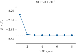
\hat f(1) = \hat h(1) + \sum_b\big[2\hat J_b(1) - \hat K_b(1)\big],

in the closed-shell case: $\hat h$ is the kinetic energy and attraction to the nuclei of one electron, $\hat J_b$ the repulsion by the charge cloud of orbital $b$ , and $\hat K_b$ the exchange operator, whose expectation values are the exchange integrals of Chapter 2. Since $\hat f$ depends on the orbitals it determines, the equations are solved by iteration until the orbitals no longer change: a self-consistent field (SCF).

Theorem 3.12 (Roothaan–Hall equations)

Writing each orbital in a basis, $\phi_a = \sum_\mu C_{\mu a}\chi_\mu$ , the closed-shell Hartree–Fock equations become the matrix eigenproblem

\mathbf F\mathbf C = \mathbf S\mathbf C\boldsymbol\varepsilon, \qquad F_{\mu\nu} = h_{\mu\nu} + \sum_{\lambda\sigma}P_{\lambda\sigma}\big[(\mu\nu|\sigma\lambda) - \tfrac12(\mu\lambda|\sigma\nu)\big],

with the density matrix $P_{\lambda\sigma} = 2\sum_a^{\mathrm{occ}}C_{\lambda a}C_{\sigma a}$ and the two-electron integrals $(\mu\nu|\lambda\sigma) = \iint\chi_\mu(1)\chi_\nu(1) r_{12}^{-1}\chi_\lambda(2)\chi_\sigma(2)$ (atomic units).

Partial proof. The energy of the determinant is $E = \sum_{\mu\nu}P_{\mu\nu}h_{\mu\nu} + \frac12 \sum P_{\mu\nu}P_{\lambda\sigma}[(\mu\nu|\sigma\lambda) - \frac12(\mu\lambda|\sigma\nu)]$ , a quadratic function of the coefficients. Minimise it under the constraints that the orbitals stay orthonormal, $\mathbf C^{\mathsf T}\mathbf S\mathbf C = \mathbf 1$ , with a Lagrange multiplier for each constraint: the stationarity conditions are $\mathbf F\mathbf C = \mathbf S\mathbf C\boldsymbol\varepsilon$ , the multipliers forming a matrix that can be made diagonal by a rotation of the occupied orbitals among themselves. The algebra is admitted. ∎

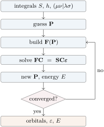
Method 3.13 (The SCF procedure)

Compute the integrals $S_{\mu\nu}$ , $h_{\mu\nu}$ and $(\mu\nu|\lambda\sigma)$ once.
Guess the density matrix (for instance from the eigenvectors of $\mathbf h$ alone, the “core” guess).
Build $\mathbf F$ from $\mathbf P$ ; solve $\mathbf F\mathbf C = \mathbf S\mathbf C \boldsymbol\varepsilon$ (orthogonalise with $\mathbf S^{-1/2}$ , then diagonalise).
Fill the lowest orbitals, two electrons each; form the new $\mathbf P$ and the energy.
Repeat from step 3 until the energy and $\mathbf P$ change by less than a threshold.

The self-consistent-field loop of a Hartree–Fock calculation.

Example 3.14 ( $\ce{H2}$ in the minimal basis)

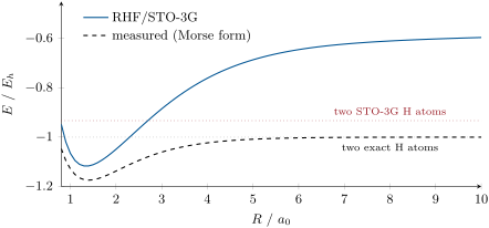
With one STO-3G function per atom, the bonding orbital is fixed by symmetry, $\sigma_g \propto \chi_A + \chi_B$ , and the SCF needs a single step. At $R = 1.4\,a_0$ the overlap is $S_{AB} = 0.6593$ and the energy $-1.1167\,E_\mathrm{h}$ ; the minimum lies at $1.346\,a_0$ ( $71.2\,\mathrm{pm}$ , against the measured $74.1\,\mathrm{pm}$ ) and $-1.1175\,E_\mathrm{h}$ . The figure below compares the curve with the true one, built from measured spectroscopic data and the dissociation energy (a Morse curve, Chapter 6).

The energy of H2 against the internuclear distance: restricted Hartree–Fock in the STO-3G basis (solid) and the true curve (dashed, Morse form built from the measured D_0, _e, _ex_e, r_e). Near the minimum RHF is good; at large R it rises far above two hydrogen atoms. — The energy of $\ce{H2}$ against the internuclear distance: restricted Hartree–Fock in the STO-3G basis (solid) and the true curve (dashed, Morse form built from the measured $D_0$ , $\omega_e$ , $\omega_ex_e$ , $r_e$ ). Near the minimum RHF is good; at large $R$ it rises far above two hydrogen atoms.

Proposition 3.15 (Why restricted Hartree–Fock fails at dissociation)

In the minimal basis, the RHF wavefunction of $\ce{H2}$ is, apart from normalisation, $\sigma_g(1)\sigma_g(2) \propto \chi_A(1)\chi_B(2) + \chi_B(1)\chi_A(2) + \chi_A(1)\chi_A(2) + \chi_B(1)\chi_B(2)$ : at any distance, half covalent and half ionic ( $\ce{H+ H-}$ ). At large $R$ its energy tends to the mean of two neutral atoms and of an ion pair, not to that of two atoms.

Proof. Expand $(\chi_A + \chi_B)(1)(\chi_A + \chi_B)(2)$ : the two cross terms put one electron on each atom, the two square terms both on the same atom, with equal weights whatever $R$ . The determinant cannot change these weights. ∎

Definition 3.16 (Electron correlation, correlation energy)

Electron correlation is the part of the electrons’ mutual avoidance not described by a single determinant (whose electrons of opposite spins move independently in each other’s average field). The correlation energy is the exact energy minus the Hartree–Fock energy in a complete basis; it is always negative.

The correlation energy is about $-0.04\,E_\mathrm{h}$ per electron pair, one per cent of a total energy but comparable to the energy of a reaction: methods that add it (configuration interaction, perturbation theory, coupled clusters) cost far more than Hartree–Fock, whose cost already grows roughly as the fourth power of the number of basis functions.

Theorem 3.17 (Koopmans’ theorem)

In Hartree–Fock theory, the energy needed to remove an electron from occupied orbital $a$ , keeping all other orbitals frozen, is $-\varepsilon_a$ . The measured ionisation energies are therefore approximately the negatives of the orbital energies: this is Koopmans’ theorem.

Proof. The energy of a closed-shell determinant is $\sum_a2h_{aa} + \sum_{ab}(2J_{ab} - K_{ab})$ , and $\varepsilon_a = h_{aa} + \sum_b(2J_{ab} - K_{ab})$ . Remove one electron from $a$ without changing the orbitals: the lost terms are $h_{aa}$ , the interactions of that electron with all others, $\sum_b(2J_{ab} - K_{ab}) - J_{aa}$ , plus $J_{aa}$ with its former partner — in total exactly $\varepsilon_a$ . So $E^+ - E = -\varepsilon_a$ . ∎

Example 3.18 (Ionising $\ce{H2}$ )

At $1.4\,a_0$ , the STO-3G orbital energy of $\sigma_g$ is $-0.5782\,E_\mathrm{h}$ : Koopmans predicts $15.73\,\mathrm{eV}$ , against the measured $15.43\,\mathrm{eV}$ . The frozen orbitals overestimate the energy of the ion (it would relax), the missing correlation acts the other way; for valence ionisations the two errors largely cancel, which is why the photoelectron spectra of the Year 2 volume can be read with orbital diagrams.

3.5 Density-functional theory, and what a calculation can tell

The wavefunction of $N$ electrons depends on $3N$ coordinates; the electron density depends on three.

Definition 3.19 (Electron density, density-functional theory)

The electron density $\rho(\mathbf r)$ is the number of electrons per unit volume at $\mathbf r$ , summed over all electrons: $\int\rho\,\dd\tau = N$ . Density-functional theory (DFT) computes the ground-state energy as a functional of $\rho$ . In practice $\rho = \sum_a|\phi_a|^2$ is built from Kohn–Sham orbitals, the orbitals of fictitious independent electrons that have the same density as the real ones, and all the effects of exchange and correlation are gathered in an exchange–correlation functional $E_{\mathrm{xc}}[\rho]$ .

Theorem 3.20 (Hohenberg–Kohn)

The ground-state density of a system of electrons determines the external potential (the nuclei) up to a constant, hence the Hamiltonian and every ground-state property; and the energy functional of the density is minimal at the true density.

Proof. Admitted at this level. ∎

The proof is treated in more advanced courses. It guarantees that an exact functional exists, not what it is: every practical functional is an approximation, chosen from a hierarchy — local density, gradient corrections, hybrids mixing in some Hartree–Fock exchange — and calibrated on reference data. The Kohn–Sham equations are solved by the same SCF loop as Hartree–Fock, at a similar cost, but include correlation; this is why DFT became the workhorse of chemistry.

Method 3.21 (Reading a calculation)

Check that the SCF converged and that the geometry optimisation ended with forces below threshold.
Run a frequency calculation at the same level: all real frequencies mean a minimum; one imaginary frequency, a transition structure, whose normal mode is the motion across the barrier.
Compare like with like: energy differences between structures computed at one level, never absolute energies from different levels.
Compare with experiment knowing the typical errors of the level: harmonic frequencies are usually scaled down by 0.9 to 0.97; bond lengths are good to about 1 pm with a hybrid functional and a polarised basis; reaction energies to a few $\mathrm{kJ}/\mathrm{mol}$ at best.

Method 3.22 (Choosing a level of theory)

Geometries and frequencies of organic molecules: a hybrid functional with a polarised split-valence basis. Weak interactions: add a dispersion correction and diffuse functions. Reaction barriers and accurate energetics: correlated wavefunction methods on DFT geometries, as far as the budget allows. Large systems (proteins, surfaces): a small region treated quantum-mechanically inside a classical force field. Always test the chosen level on a related molecule whose answer is known.

In the lab — A computational experiment

A calculation is run like an experiment and recorded in the notebook: the program and its version, the method, the basis, the convergence thresholds, the starting structure, and the output files kept as raw data. A typical sequence is: build the molecule, optimise its geometry at a modest level, compute frequencies to confirm a minimum, then compute the energy at a higher level on that geometry.

History — A molecule known first by calculation

$\ce{HeH+}$ was produced in the laboratory in 1925. Its properties were computed in detail from the 1930s onwards, and it was predicted to be abundant in some astrophysical gases; but its first rotational line lies in the far infrared, absorbed by the atmosphere. In 2019 an airborne observatory detected it in the planetary nebula NGC 7027, at the frequency calculations and laboratory spectra had predicted.

3.6 Exercises

Exercise 3.1 ★

For the hydrogen atom, take the trial function $\eu^{-\alpha r^2}$ . In atomic units $E(\alpha) = \frac32\alpha - 2\sqrt{2\alpha/\pi}$ . Find the best $\alpha$ and the corresponding energy; compare with $-\frac12E_h$ .

Solution

Solution of Exercise 3.1.

$\dd E/\dd\alpha = \frac32 - \sqrt{2/\pi\alpha} = 0$ gives $\alpha = 8/9\pi = 0.283\, a_0^{-2}$ and $E = \frac32\alpha - 2\sqrt{2\alpha/\pi} = -4/3\pi = -0.4244\,E_\mathrm{h}$ , 15 % above the exact $-0.5$ : a single Gaussian has neither the cusp nor the tail of the $1s$ function.

Exercise 3.2 ★

How many basis functions does a calculation on benzene use in the STO-3G basis? In 6-31G(d), with six Cartesian $d$ functions per carbon and two $s$ functions per hydrogen?

Solution

Solution of Exercise 3.2.

STO-3G: 5 functions per C ( $1s$ , $2s$ , three $2p$ ) and 1 per H: $6 \times 5 + 6 = 36$ . 6-31G(d): per C, 1 (core) + $2 \times 4$ (split valence) + 6 ( $d$ ) $= 15$ ; per H, 2: $6 \times 15 + 6 \times 2 = 102$ .

Exercise 3.3 ★

Explain why $\ce{H2}$ and $\ce{D2}$ have the same bond length and the same force constant but different vibrational wavenumbers. Which ratio do you expect?

Solution

Solution of Exercise 3.3.

The electronic Hamiltonian does not contain the nuclear masses: within the Born–Oppenheimer approximation the PES, hence $r_e$ and $k = U''(r_e)$ , is the same. $\tilde\omega = \sqrt{k/\mu}/2\pi c$ depends on the reduced mass, which doubles: ratio $\sqrt2 = 1.414$ (measured 1.413).

Exercise 3.4 ★

A frequency calculation on a structure of formula $\ce{C2H5F}$ gives 17 real frequencies and one imaginary frequency, $487\iu$ $\mathrm{cm}^{-1}$ . What kind of stationary point is it? How many frequencies did you expect in total?

Solution

Solution of Exercise 3.4.

Eight atoms give $3N - 6 = 18$ vibrations: 17 real and one imaginary. One negative Hessian eigenvalue: a first-order saddle point, a transition structure (here, for example, of a rotation or an elimination).

Exercise 3.5 ★★

Using $E(\zeta) = \zeta^2 - \frac{27}{8}\zeta$ , compute the best variational energy of helium in $E_\mathrm{h}$ and eV, and its error against the exact $-2.9034\,E_\mathrm{h}$ . What fraction of the total energy is the error?

Solution

Solution of Exercise 3.5.

$\zeta = 27/16$ , $E = -(27/16)^2 = -2.8477\,E_\mathrm{h} = -77.49\,\mathrm{eV}$ . Error $-2.8477 + 2.9034 = 0.0557\,E_\mathrm{h} = 1.52\,\mathrm{eV}$ , that is 1.9 % of the total energy — but larger than many reaction energies.

Exercise 3.6 ★★

Two basis functions give $H_{11} = -1.0\,E_\mathrm{h}$ , $H_{22} = -0.5\,E_\mathrm{h}$ , $H_{12} = -0.2\,E_\mathrm{h}$ , $S_{12} = 0.3$ . Solve the secular equation. Is the lower root below $H_{11}$ ?

Solution

Solution of Exercise 3.6.

$(-1 - E)(-0.5 - E) - (-0.2 - 0.3E)^2 = 0$ , i.e. $0.91E^2 + 1.38E + 0.46 = 0$ : $E = -1.0217\,E_\mathrm{h}$ and $-0.4947\,E_\mathrm{h}$ . Yes: mixing in the second function lowers the energy below $H_{11}$ , as the variational principle allows.

Exercise 3.7 ★★

A Hartree–Fock calculation takes 10 minutes for benzene in STO-3G. Assuming a cost proportional to the fourth power of the number of basis functions, estimate the time in 6-31G(d).

Solution

Solution of Exercise 3.7.

$(102/36)^4 = 64$ : about 640 minutes, some 11 hours.

Exercise 3.8 ★★

The STO-3G orbital energy of $\ce{H2}$ at $1.4\,a_0$ is $-0.5782\,E_\mathrm{h}$ . Give Koopmans’ estimate of the ionisation energy in eV and compare with $15.43\,\mathrm{eV}$ . Name two reasons why they differ and their directions.

Solution

Solution of Exercise 3.8.

$0.5782 \times 27.211 = 15.73\,\mathrm{eV}$ , 0.30 eV above the measured value. Frozen orbitals: the real ion relaxes and is lower, so Koopmans’ value is too high. Missing correlation: the neutral molecule (two electrons) has more correlation energy than the ion (one electron), which makes the true value larger. Here the first error wins.

Exercise 3.9 ★★

In STO-3G, the energy of one hydrogen atom is $-0.4666\,E_\mathrm{h}$ and the RHF energy of $\ce{H2}$ at $10\,a_0$ is $-0.5960\,E_\mathrm{h}$ . How far above two atoms is the RHF energy at that distance, in eV? Explain with the ionic terms.

Solution

Solution of Exercise 3.9.

$-0.5960 - 2(-0.4666) = 0.3372\,E_\mathrm{h} = 9.18\,\mathrm{eV}$ above two atoms. The RHF function keeps 50 % of $\ce{H+ H-}$ , and separating a proton and a hydride costs the difference between the ionisation energy of H and the electron affinity of H, which the energy averages in.

Exercise 3.10 ★★★

For $\phi = c_1\chi_1 + c_2\chi_2$ with real functions, write $E(c_1,c_2)$ and derive the two secular equations by setting $\partial E/\partial c_1 = \partial E/\partial c_2 = 0$ .

Solution

Solution of Exercise 3.10.

$E(c_1^2 + 2c_1c_2S + c_2^2) = c_1^2H_{11} + 2c_1c_2H_{12} + c_2^2H_{22}$ . Differentiating with respect to $c_1$ with $\partial E/\partial c_1 = 0$ : $E(2c_1 + 2c_2S) = 2c_1H_{11} + 2c_2H_{12}$ , i.e. $(H_{11} - E)c_1 + (H_{12} - ES)c_2 = 0$ ; similarly $(H_{12} - ES)c_1 + (H_{22} - E)c_2 = 0$ .

Exercise 3.11 ★★★

The RHF/STO-3G energy of $\ce{H2}$ is $-1.116871$ , $-1.117501$ and $-1.116\,714\,E_\mathrm{h}$ at $R = 1.30$ , 1.35 and $1.40\,a_0$ . Estimate the force constant by a finite difference, convert it to $\mathrm{N}/\mathrm{m}$ ( $1\,E_\mathrm{h}/{a_0}^{2} = 1556.9\,\mathrm{N}/\mathrm{m}$ ), and compute the harmonic wavenumber. Compare with $\tilde\omega_e = 4401\,\mathrm{cm}^{-1}$ .

Solution

Solution of Exercise 3.11.

$k \approx [E(1.30) - 2E(1.35) + E(1.40)]/(0.05)^2 = 0.001417/0.0025 = 0.567\,E_\mathrm{h}/{a_0}^{2} = 882\,\mathrm{N}/\mathrm{m}$ . With $\mu = m_H/2 = 8.37 \times 10^{-28}\,\mathrm{kg}$ , $\omega = \sqrt{k/\mu} = 1.03 \times 10^{15}\,\mathrm{s}^{-1}$ and $\tilde\omega = \omega/2\pi c = 5452\,\mathrm{cm}^{-1}$ , 24 % above the measured $\tilde\omega_e$ : a minimal-basis RHF curve is too steep (no correlation, too small a basis), which is why computed frequencies are scaled down.

Exercise 3.12 ★★★

You must compute the energy difference between two conformers of a sugar, known to differ by a few $\mathrm{kJ}/\mathrm{mol}$ , with an intramolecular hydrogen bond in one of them. Choose and justify a method, a basis set and the checks you would run.

Solution

Solution of Exercise 3.12.

Differences of a few $\mathrm{kJ}/\mathrm{mol}$ involving a hydrogen bond need correlation and dispersion: a hybrid functional with a dispersion correction, or better a correlated wavefunction method for the final energies, with a polarised triple-split basis including diffuse functions. Optimise both conformers at the same level, confirm minima by frequencies (all real), add zero-point energies, test the basis by one larger calculation, and compare with a related system of known conformational energy.

3.7 Problem: HeH $^+$ , the First Molecule

Problem 3.1

Weekend problem — a minimal-basis Hartree–Fock calculation of the helium hydride ion: the basis, the core guess, the converged orbital, and the binding of a proton to helium

$\ce{HeH+}$ is computed at $R = 1.4632\,a_0$ in the STO-3G basis (He exponents 6.3624, 1.1589, 0.31365; H exponents 3.4253, 0.62391, 0.16886; the same three coefficients). Function 1 is on He, function 2 on H. The program gives (atomic units)

\mathbf S = \begin{pmatrix}1 & 0.5368\\ 0.5368 & 1\end{pmatrix},\quad \mathbf h = \begin{pmatrix}-2.5983 & -1.4318\\ -1.4318 & -1.7318\end{pmatrix},\quad \mathbf F_{\mathrm{final}} = \begin{pmatrix}-1.5902 & -1.0610\\ -1.0610 & -0.8340 \end{pmatrix},

the occupied orbital $\phi = 0.8766\chi_1 + 0.2025\chi_2$ , the orbital energies $-1.6328$ and $-0.1725\,E_\mathrm{h}$ , and the SCF energies $-2.7978$ , $-2.8404$ , $-2.8418$ , $-2.8418$ . A helium atom in the same basis has $-2.8078\,E_\mathrm{h}$ . $1\,E_\mathrm{h} = 27.211\,\mathrm{eV} = 2625.5\,\mathrm{kJ}/\mathrm{mol}$ .

Part I — The basis.

What does “STO-3G” mean?
Why are the helium exponents larger than the hydrogen ones? Check that their ratio is $(1.69/1.24)^2$ .
How many basis functions, electrons and occupied orbitals are there?
Compute the nuclear repulsion energy.
Interpret $S_{12} = 0.5368$ .
Why is $h_{11}$ lower than $h_{22}$ ?

Part II — The core guess.

Write the secular equation $\det(\mathbf h - \varepsilon\mathbf S) = 0$ as a quadratic in $\varepsilon$ .
Solve it.
Why is this only a starting point?
Give the formula of the Fock matrix in terms of $\mathbf h$ , the density matrix and the two-electron integrals.
Which electron interactions does $\mathbf F$ contain that $\mathbf h$ lacks?
Explain why the procedure must be iterated.

Part III — The converged orbital.

Check that $\phi$ is normalised.
The populations are $P\mathbf S$ diagonal elements, $2c_1^2 + 2c_1c_2S$ on He and $2c_2^2 + 2c_1c_2S$ on H. Compute them.
Where does the positive charge sit? Is the molecule better described as $\ce{He + H+}$ or $\ce{He+ + H}$ ?
Use Koopmans’ theorem to estimate the energy needed to remove an electron from $\ce{HeH+}$ .
Compute the electronic energy $E_{\mathrm{el}} = E - V_{\mathrm{nn}}$ .
How many cycles were needed to converge to $10^{-4}\,E_\mathrm{h}$ ? Why did the energy decrease at each cycle?
With helium exponents scaled to $\zeta = 2.0925$ instead of 1.69, the same program gives $-2.8607\,E_\mathrm{h}$ . Which basis is better, and why can you say so?
What does the virtual orbital energy, $-0.1725\,E_\mathrm{h}$ , represent?

Part IV — The binding of a proton.

What is the energy of a bare proton? Of $\ce{He + H+}$ far apart, in this basis?
Compute the energy released by $\ce{He + H+ -> HeH+}$ at this level, in $\mathrm{kJ}/\mathrm{mol}$ .
The measured proton affinity of helium is $177.8\,\mathrm{kJ}/\mathrm{mol}$ . Comment.
The exact energy of helium is minus the sum of its ionisation energies, 24.5874 and $54.4178\,\mathrm{eV}$ . Compute it in $E_\mathrm{h}$ and the error of the STO-3G helium atom.
Why can an error of this size still give useful molecular geometries?
State the result: the RHF/STO-3G total energy of $\ce{HeH+}$ at $1.4632\,a_0$ .

Solution

Solution of Problem 3.1.

1. Each Slater-type orbital of a minimal basis is replaced by a fixed contraction of three Gaussians fitted to it. 2. The helium nucleus attracts its electrons more, so its $1s$ function is more compact (larger exponents). $6.3624/3.4253 = 1.857 = (1.69/1.24)^2$ . 3. Two basis functions, two electrons, one occupied orbital (and one virtual). 4. $V_{\mathrm{nn}} = Z_{\mathrm{He}}Z_{\mathrm H}/R = 2/1.4632 = 1.3669\,E_\mathrm{h}$ . 5. The two functions overlap strongly (54 %): the atoms are close enough to bond. 6. $h_{11}$ is the energy of an electron in the He function with both nuclei but no other electron; the He nucleus (charge 2) holds it much more tightly. 7. $(h_{11} - \varepsilon)(h_{22} - \varepsilon) - (h_{12} - \varepsilon S)^2 = 0$ : $0.71185\varepsilon^2 + 2.79292\varepsilon + 2.44969 = 0$ . 8. $\varepsilon = -2.600\,E_\mathrm{h}$ and $-1.324\,E_\mathrm{h}$ . 9. $\mathbf h$ ignores the repulsion between the two electrons; the core orbital is too contracted and too low. 10. $F_{\mu\nu} = h_{\mu\nu} + \sum_{\lambda\sigma}P_{\lambda\sigma}[(\mu\nu|\sigma\lambda) - \frac12(\mu\lambda|\sigma\nu)]$ , with $P_{\lambda\sigma} = 2C_{\lambda1}C_{\sigma1}$ . 11. The Coulomb repulsion of each electron by the charge cloud of the other (and, in general, exchange). 12. $\mathbf F$ depends on $\mathbf P$ , which depends on the orbitals obtained from $\mathbf F$ : the equations are non-linear and are solved by successive approximations until self-consistency. 13. $c_1^2 + c_2^2 + 2c_1c_2S = 0.7684 + 0.0410 + 0.1906 = 1.0000$ . 14. He: $1.5369 + 0.1906 = 1.727$ ; H: $0.0820 + 0.1906 = 0.273$ electron. 15. Charges: He $+0.27$ , H $+0.73$ . The positive charge sits mostly on hydrogen: $\ce{HeH+}$ is a proton bound to a helium atom, $\ce{He + H+}$ , as expected since the ionisation energy of He (24.6 eV) far exceeds that of H (13.6 eV). 16. $-\varepsilon_1 = 1.633\,E_\mathrm{h} = 44.4\,\mathrm{eV}$ . 17. $E_{\mathrm{el}} = -2.8418 - 1.3669 = -4.2087\,E_\mathrm{h}$ . 18. Three cycles reach $-2.8418\,E_\mathrm{h}$ . Each cycle gives a determinant, whose energy is an upper bound to the converged Hartree–Fock energy (variational principle), and the iterations improve it. 19. The basis with $\zeta = 2.0925$ gives the lower energy, so it is the better one for this molecule (variational principle): the helium function is more compact in $\ce{HeH+}$ than in the free atom, whose $\zeta = 1.69$ the standard basis copies. 20. The empty antibonding orbital $\sigma^*$ ; its energy would approximate minus the electron affinity of $\ce{HeH+}$ (poorly, in such a small basis). 21. Zero (no electron); $-2.8078\,E_\mathrm{h}$ . 22. $-2.8078 - (-2.8418) = 0.0340\,E_\mathrm{h} = 89\,\mathrm{kJ}/\mathrm{mol}$ . 23. About half the measured value: a minimal basis cannot polarise the helium density towards the proton (there are no $p$ functions), so the bond is too weak. (Zero-point and $298\,\mathrm{K}$ corrections are small beside this.) 24. $-(24.5874 + 54.4178)/27.211 = -2.9034\,E_\mathrm{h}$ ; the STO-3G atom is $0.0956\,E_\mathrm{h}$ ( $2.6\,\mathrm{eV}$ ) too high. 25. Geometries depend on how the energy changes with $R$ ; most of the error, concentrated in the core, is nearly the same at every geometry and cancels. 26. $E(\ce{HeH+}) = -2.8418\,E_\mathrm{h}$ at RHF/STO-3G (standard basis), $1.4632\,a_0$ (and $-2.8607\,E_\mathrm{h}$ with the classic $\zeta_{\mathrm{He}} = 2.0925$ ).

Terms defined in this chapter

See all 852 terms in the glossary

3.1 Born–Oppenheimer and the potential energy surface

3.2 The variational principle

3.3 Basis sets

3.4 Hartree–Fock theory

3.5 Density-functional theory, and what a calculation can tell

3.6 Exercises

3.7 Problem: HeH+^++, the First Molecule

Terms defined in this chapter

3.7 Problem: HeH $^+$ , the First Molecule