The tomb of Ludwig Boltzmann in Vienna carries a single line, S=klogW: the entropy of a system counts the ways its molecules can share out its energy. Thermodynamics, as the Year 1 and Year 2 volumes built it, never needs molecules: it relates measured heats, entropies and equilibrium constants to one another. Statistical thermodynamics computes them from the molecules themselves. Its central object is a single sum over the energy levels of one molecule, the partition function; the levels come from spectroscopy, and the standard entropy of nitrogen computed from its spectrum agrees with the tabulated value to a hundredth of a joule per kelvin and per mole. This chapter builds the partition function, splits it into its translational, rotational, vibrational and electronic parts, and turns it into internal energy, entropy and Gibbs energy; Chapter 11 applies it to heat capacities and equilibrium constants.
You already know
The Year 2 volume defined the standard molar entropy, the Gibbs energy and the chemical potential, and tabulated entropies obtained from heat capacities measured down to low temperature. Chapter 1 gave the energy levels of a particle in a box, of the harmonic oscillator and of the rigid rotor, EJ=hcBJ(J+1) with degeneracy2J+1; Chapter 6 measured B and ν~ for diatomic molecules and found that in a homonuclear molecule such as NX2 the nuclear spins make alternate rotational levels unequal.
10.1 Microstates and the Boltzmann distribution
Consider N identical, independent molecules that can occupy levels of energy ε0=0<ε1<ε2<…, with total energy E. Saying how many molecules are on each level, {n0,n1,…}, describes a distribution; saying which molecule is on which level describes much more.
Definition 10.1(Microstate, statistical weight)
A microstate of a system of molecules is a complete specification of the state of every molecule. The statistical weightW of a distribution {ni} of N molecules over non-degenerate levels is the number of microstates that realise it:
W=n0!n1!n2!⋯N!.
Example 10.2(Three quanta among three oscillators)
Three oscillators share three quanta of energy. The distribution “one oscillator holds all three” can be realised in 3!/(1!2!)=3 ways, “one holds two, another one” in 3!=6 ways and “each holds one” in one way: ten microstates in all, and the most even distribution that still spreads the energy over several levels is the most probable. With 1023 molecules the weights become so sharply peaked that one distribution, and the ones that differ from it by a negligible amount, carry practically all the microstates.
Remark 10.3
The postulate of statistical thermodynamics is that all the microstates of an isolated system with a given energy are equally probable. The system is then found, overwhelmingly, in the distribution of largest weight: finding it is the task of this section.
For large numbers, Stirling’s approximation lnx!≈xlnx−x gives
The populationni/N of a level is the fraction of the molecules that occupy it. The Boltzmann distribution is the distribution of largest weight of independent molecules at thermal equilibrium at temperature T, given by the theorem below.
Theorem 10.5(The Boltzmann distribution)
For independent molecules at equilibrium at temperature T, the population of a level of energy εi and degeneracygi is
Nni=qgie−εi/kT,q=i∑gie−εi/kT,
where k is the Boltzmann constant. Two levels have populations in the ratio ninj=gigje−(εj−εi)/kT.
Partial proof. Take first non-degenerate levels. Maximise lnW under the two constraints ∑ini=N and ∑iniεi=E with Lagrange multipliers α and β: for every i,
∂ni∂(lnW+αj∑nj−βj∑njεj)=−lnni−1+α−βεi=0,
so ni=eα−1e−βεi, and the first constraint fixes eα−1=N/∑je−βεj. A level of degeneracygi is gi distinct states of the same energy, each populated as above: its population is multiplied by gi. The multiplier β is identified by one known case: for the translational motion of an ideal gas (Proposition 10.11 below) the distribution gives an energy 23N/β, and the ideal-gas energy is 23NkT; hence β=1/kT. That β is the same quantity for every kind of motion, and that it is the thermodynamic temperature, is admitted here: two systems in thermal contact share the same β, which is the defining property of temperature. ∎
Definition 10.6(Molecular partition function)
The molecular partition function of a molecule at temperature T is the sum
q=levels∑gie−εi/kT=states∑e−εs/kT,
with energies measured from the lowest level, so that q≥1.
The partition function counts the states that are thermally accessible: at very low temperature only the lowest level contributes and q→g0; at very high temperature every state contributes about 1 and q grows without limit. A rule of thumb follows: levels much more than kT above the lowest one are empty, levels within kT of it are populated. At 298.15K, kT corresponds to 207.2cm−1, or RT=2.479kJ/mol.
Method 10.7(Populations of levels from spectroscopic constants)
List the levels with their energies (from the constants, e.g. hcBJ(J+1)) and degeneracies (2J+1).
Express each energy in units of kT; at 298.15K, divide a wavenumber by 207.2cm−1.
Form the terms gie−εi/kT, add them up to get q, and divide. Stop the sum when the terms are negligible.
Check: the populations add up to 1; the ratio of two of them is gigje−(εj−εi)/kT.
Example 10.8(The rotational levels of hydrogen chloride)
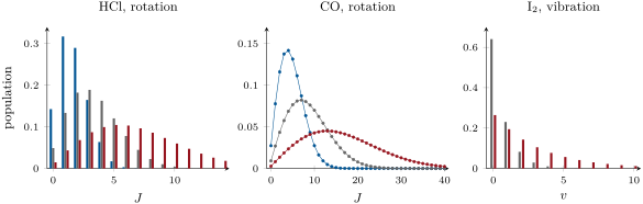
For HX35X2235Cl, B0=Be−αe/2=10.44cm−1. At 300K the level J lies at 10.44J(J+1)cm−1, i.e. 0.0501J(J+1) in units of kT. The terms (2J+1)e−0.0501J(J+1) are 1, 2.71, 3.70, 3.84, 3.31, 2.45, …; their sum is q=20.3 and the populations of J=0 to 4 are 0.049, 0.134, 0.182, 0.189 and 0.163: the most populated level is J=3, not J=0, because the degeneracy2J+1 grows while the Boltzmann factor falls. This is the envelope of the rotation–vibration band of Chapter 6.
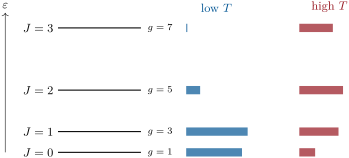
A Boltzmann staircase: rotational levels J=0 to 3 (energies 0, 2, 6, 12 times hcB, degeneracies 2J+1) and their populations, as bar lengths, at kT=2hcB and kT=10hcB (the four levels alone). Heating empties the lowest level towards the upper ones; at both temperatures the bars add up to the same total, the number of molecules.
10.2 The molecular partition function
Proposition 10.9(Factorisation)
If the energy of a molecule is a sum of independent contributions, ε=εT+εR+εV+εE, each state being any combination of a translational, a rotational, a vibrational and an electronic state, then
q=qTqRqVqE.
Proof. The sum over all combinations of an exponential of a sum is the product of the separate sums: ∑a,be−(εa+εb)/kT=(∑ae−εa/kT)(∑be−εb/kT), and likewise for four factors. ∎
The separation is an approximation: rotation and vibration interact (the constant αe), and the electronic state sets the rotational and vibrational constants. For a molecule in its ground electronic state at ordinary temperatures the errors are a few hundredths of a joule per kelvin in an entropy. The populations are then computed separately for each kind of motion: the fraction of molecules in a vibrational level v does not depend on their rotation.
10.3 The four contributions
Translation
Definition 10.10(Thermal wavelength)
The thermal wavelength of a molecule of mass m at temperature T is Λ=2πmkTh.
For a molecule of mass m free to move in a volume V,
qT=Λ3V.
Proof. For one dimension, a box of length L has levels εn=h2n2/8mL2 (n=1,2,…; the zero-point offset changes nothing measurable). They are so close together that the sum is an integral:
The three directions are independent: qT=qxqyqz=L3/Λ3. The mean energy per dimension is −∂lnqx/∂β with qx∝β−1/2, that is 1/2β; three dimensions give 23kT per molecule, as used in the proof of Theorem 10.5. ∎
Example 10.12(Argon in a flask)
For argon (M=39.95g/mol) at 298.15K, Λ=16.0pm, a tenth of an atomic diameter. In 1dm3, qT=10−3/(1.600×10−11)3=2.44×1029 translational states are thermally accessible, far more than the 2.4×10²² atoms the flask holds at 1bar: each state is almost always empty, the condition under which the molecules can be counted as below.
Rotation
Definition 10.13(Characteristic temperatures)
The characteristic rotational temperature of a linear molecule of rotational constantB is θR=hcB/k; the characteristic vibrational temperature of a vibration of wavenumber ν~ is θV=hcν~/k.
Definition 10.14(Symmetry number)
The symmetry numberσ of a molecule is the number of distinct orientations of the rigid molecule that are reached by proper rotations and are indistinguishable from the starting one (the order of the rotational subgroup of its point group): 1 for HCl and CO, 2 for NX2, COX2 and HX2O, 3 for NHX3, 12 for CHX4 and CX6HX6.
Proposition 10.15(Rotational partition function)
For a linear molecule, qR=∑J(2J+1)e−θRJ(J+1)/T. When T≫θR,
qR≈σθRT=σhcBkT,
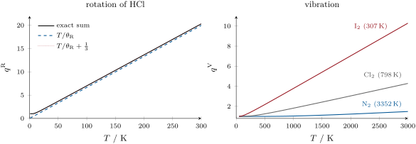
with a relative error of about θR/3T for σ=1 (the exact sum is close to T/θR+31).
Partial proof. For T≫θR many levels contribute and the sum becomes an integral. With x=J(J+1), dx=(2J+1)dJ:
∫0∞(2J+1)e−θRJ(J+1)/TdJ=∫0∞e−θRx/Tdx=θRT.
The correction 31 comes from the next term of the Euler–Maclaurin formula (Exercise 10.11). The factor 1/σ is admitted here and justified in Chapter 11: in a homonuclear molecule the symmetry of the wavefunction under the exchange of the two identical nuclei allows each nuclear-spin state only one parity of J (Chapter 6), so on average half the rotational levels are missing. Counting the rotational states with σ in this way leaves the nuclear-spin states out of q; the thermodynamic tables follow the same convention, and the nuclear-spin factor cancels in every chemical reaction. ∎
For NX2, B0=1.990cm−1 and θR=2.86K: at 298.15K, qR=298.15/(2×2.863)=52.1. For HCl, θR=15.0K and qR=19.8 (exact sum 20.2). Only HX2 (θR=85K) and its isotopologues need the exact sum at room temperature. A non-linear molecule with rotational constantsA, B, C has qR=σ1(hckT)3/2ABCπ, admitted.
Vibration
Proposition 10.16(Vibrational partition function)
For a harmonic vibration of wavenumber ν~, with energies measured from the zero-point level,
qV=v≥0∑e−vθV/T=1−e−θV/T1.
It tends to 1 when T≪θV and to T/θV when T≫θV. A molecule with several normal modes has the product of one such factor per mode.
Proof. The levels are vhcν~ above the zero-point level: the sum is a geometric series of ratio e−θV/T<1. When T≫θV, 1−e−θV/T≈θV/T. The normal modes are independent (Proposition 10.9). ∎
For the vibrational quantum of a diatomic molecule this book takes the observed fundamental G(1)−G(0)=ωe−2ωexe (Chapter 6); at room temperature only the first levels matter, and their spacing is what counts. Stiff, light molecules are frozen: NX2 has θV=3352K, qV=1.000013 at 298.15K, and only 13 molecules in a million are in v=1. Heavy, soft ones are not: IX2 has θV=307K, qV=1.556, and more than a third of its molecules vibrate.
Boltzmann populations computed from the spectroscopic constants: rotational levels of HX35X2235Cl (θR=15.0K) and of CO (θR=2.77K; points joined for legibility) at 100K (blue), 300K (grey) and 1000K (red), and vibrational levels of IX2 (θV=307K) at 300 and 1000K. Rotational populations peak at J>0; vibrational ones always decrease with v, since the levels are not degenerate.
Electronic states
Proposition 10.17(Electronic partition function)
With the electronic levels εj (degeneracygj) measured from the ground level,
qE=g0+g1e−ε1/kT+⋯
For most molecules the first excited electronic level lies tens of thousands of wavenumbers up and qE=g0: 1 for a closed-shell molecule, 3 for OX2 (ground term 3Σg−), 2J+1 for an atom in a level J.
This is the definition applied to the electronic levels; the cases where low levels matter are atoms and radicals with a fine structure.
Example 10.18(Nitric oxide and the chlorine atom)
NO has a 2Π ground term split by spin–orbit coupling into 2Π1/2 (lower) and 2Π3/2, 119.73cm−1 higher, each doubly degenerate. At 298.15K, qE=2+2e−119.73/207.22=2+2×0.561=3.12: 36 % of the molecules are in the upper component. The chlorine atom has its 2P1/2 level 882.35cm−1 above the 2P3/2 ground level: qE=4+2e−4.258=4.03.
Left: the rotational partition function of HCl (θR=15.0K), exact sum against the high-temperature form; the form with the correction 31 is indistinguishable from the sum above about 30K. Right: the vibrational partition function of three diatomic molecules (characteristic temperatures in brackets), 1 while T≪θV, then close to T/θV.
10.4 From partition functions to thermodynamics
Theorem 10.19(Internal energy)
For N independent molecules, the internal energy measured from its value at T=0 is
U−U(0)=NkT2(∂T∂lnq)V=−N(∂β∂lnq)V.
The contributions of the four kinds of motion add up.
Proof.U−U(0)=∑iniεi=qN∑igiεie−βεi=−qN∂β∂q; and dβ=−dT/kT2. The volume is held fixed because the translational levels depend on it. By Proposition 10.9, lnq is a sum of four terms. ∎
For translation, qT∝T3/2 gives 23NkT; for the rotation of a linear molecule at high temperature, qR∝T gives NkT; a vibration gives NkθV/(eθV/T−1), which is NkT only when T≫θV. The classical equipartition of energy, 21kT per quadratic term, is the high-temperature limit of these results; Chapter 11 follows the heat capacities as each motion freezes out.
Definition 10.20(Canonical partition function)
The canonical partition function of a system at temperature T and volume V is the sum Q=∑se−Es/kT over all the states s of the whole system, of energies Es.
Proposition 10.21(Canonical partition function of an ideal gas)
For N independent molecules, Q=qN if they are distinguishable (localised in a crystal), and Q=qN/N! for an ideal gas of identical molecules.
Partial proof. A state of the system is a choice of state for each molecule and the energies add up: the sum of the products is the product of the sums, qN. In a gas the molecules are indistinguishable: permuting them gives the same state of the system. When the molecular states are far more numerous than the molecules (Example 10.12), almost every term of qN has its N molecules in different states and is counted N! times. Cases where two molecules share a state, which this counting gets wrong, are negligible except at very low temperature or very high density, where quantum statistics take over (admitted). ∎
Definition 10.22(Statistical entropy)
The statistical entropy of an isolated system is S=klnW, where W is the number of its microstates; for a system at temperature T, W is the weight of the dominant distribution.
For an ideal gas this gives pV=NkT and G−G(0)=−NkTln(q/N).
Partial proof. For distinguishable molecules in the Boltzmann distribution, with ni=Ngie−βεi/q and Stirling’s formula, the weight W=N!∏igini/ni! gives
so klnW=klnqN+(U−U(0))/T; for a gas, qN becomes qN/N!. The identification of klnW with the thermodynamic entropy is admitted: it is additive, maximal at equilibrium for an isolated system, and gives back the ideal-gas relations. Then A=U−TS gives the second formula, p=−(∂A/∂V)T the third: with Q=qN/N! and q∝V, p=NkT/V. Finally G=A+pV=−kTln(qN/N!)+NkT=−NkTln(q/N), using lnN!=NlnN−N. ∎
Theorem 10.24(Sackur–Tetrode equation)
The molar entropy of a monatomic ideal gas of molar mass M at temperature T and pressure p is
Sm=R[ln(pΛ3kT)+25],Λ=2πmkTh,m=NAM.
Proof. With Q=qN/N!, q=V/Λ3 and U−U(0)=23NkT, Theorem 10.23 gives S=23Nk+Nklnq−k(NlnN−N)=Nk[lnNΛ3V+25]. For one mole, Nk=R and V/N=kT/p. ∎
For argon at 298.15K and 1bar, kT/p=4.116×10−26m3 and Λ=1.600×10⁻¹¹m: Sm=R(ln1.005×107+2.5)=154.85JK−1mol−1. The tabulated standard entropy, obtained from heat capacities measured down to a few kelvins, is 154.846±0.003: the formula has no adjustable parameter, and it contains Planck’s constant. A heavier atom has a larger entropy (more translational states at the same energy), and so has a gas at lower pressure (more volume per atom).
Proposition 10.25(Rotational and vibrational molar entropies)
For a linear molecule with T≫θR, and a vibration with x=θV/T,
SmR=R[lnσθRT+1],SmV=R[ex−1x−ln(1−e−x)],
and an electronic ground level of degeneracyg0, alone populated, adds Rlng0.
Proof. For internal motions the factor 1/N! belongs to translation only, so each internal mode contributes S=TU−U(0)+Nklnq. Rotation: q=T/σθR and U−U(0)=NkT. Vibration: lnq=−ln(1−e−x) and (U−U(0))/T=Nkx/(ex−1). Electronic: q=g0, U−U(0)=0. ∎
Method 10.26(The standard entropy of a gas from its constants)
Translation: Sackur–Tetrode with the molar mass, T=298.15K and p∘=1bar.
Rotation: B0=Be−αe/2, θR=hcB0/k, the symmetry number, and R[ln(T/σθR)+1] (or the exact sum if T<30θR).
Vibration: one term per normal mode, with the fundamental wavenumbers.
Electronic: Rlng0, or R[lnqE+⟨ε⟩/kT] if low levels exist.
Add; compare with the table, where nuclear spin is left out in the same way.
gas
ST
SR
SV
SE
sum
table
Ar
154.85
0.00
0.00
0.00
154.85
154.85
NX2
150.42
41.18
0.00
0.00
191.60
191.61
CO
150.42
47.23
0.00
0.00
197.65
197.66
HCl
153.71
33.16
0.00
0.00
186.87
186.90
ClX2
162.00
58.65
2.24
0.00
222.89
223.08
IX2
177.91
74.24
8.43
0.00
260.58
260.69
Cl
153.36
0.00
0.00
11.83
165.19
165.19
Statistical standard molar entropies at 298.15K and 1bar, in JK−1mol−1, from the spectroscopic constants, against the tabulated values.
The sums agree with the tables to better than 0.2 JK−1mol−1, and to a few hundredths for the light molecules. The small residuals of ClX2 and IX2 come from approximations this chapter made: the constants of the main isotopologue, the harmonic oscillator for a molecule with many vibrational levels populated. The tabulated entropy of CO is itself the statistical value: measured calorimetrically, it comes out several JK−1mol−1 lower, a discrepancy explained in Chapter 11.
In the lab— Measuring a third-law entropy
The calorimetric route heats a sample from a few kelvins to 298.15K in an adiabatic calorimeter, measuring its heat capacity in small steps. The entropy is the sum of ∫CpdT/T over each phase, plus ΔH/T at every transition (solid–solid, fusion, vaporisation), plus a small correction for the non-ideality of the real gas; below the lowest measured temperature, Cp of a non-metallic solid is extrapolated as aT3. The third law fixes the entropy of the perfect crystal at 0 K to zero. Agreement with the statistical value, within the uncertainty of the measurement, both tests the third law and reveals the crystals that are not perfect at 0 K.
History— Boltzmann, 1877
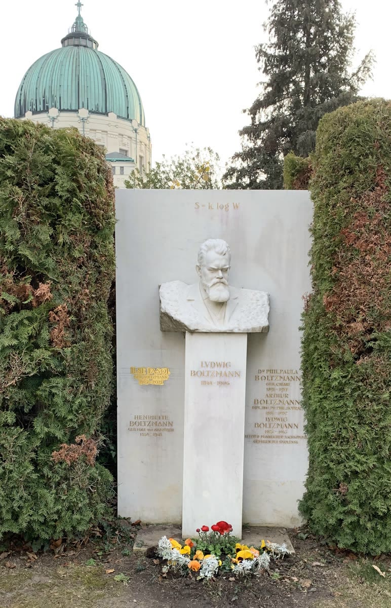
The tomb of Boltzmann.
Ludwig Boltzmann showed in 1877 that the entropy of a gas is proportional to the logarithm of the number of ways its molecules can share the energy, and derived the distribution that bears his name by counting those ways. The interpretation was fiercely contested by physicists who doubted the existence of atoms. The formula in the form S=klogW, with the constant k, was written by Max Planck, who used the same counting in 1900 for the radiation of a hot body; it is carved on Boltzmann’s tomb in the central cemetery of Vienna.
10.5 Exercises
Exercise 10.1★
Four oscillators share four quanta. List the distributions, give the weight of each, and check that they add up to the number of ways of placing four indistinguishable quanta in four oscillators, (37). Which distributions are the most probable?
Solution
Solution of Exercise 10.1.
Write each distribution as the quanta held by the four oscillators, largest first. “4, 0, 0, 0”: 4!/(3!1!)=4; “3, 1, 0, 0”: 4!/(2!1!1!)=12; “2, 2, 0, 0”: 4!/(2!2!)=6; “2, 1, 1, 0”: 4!/(1!2!1!)=12; “1, 1, 1, 1”: 1. Total 35 =(37). The most probable are “3, 1, 0, 0” and “2, 1, 1, 0” (12 each); the second, with populations 1, 2, 1 for 0, 1, 2 quanta, already falls off with energy as the Boltzmann distribution does for large numbers.
Exercise 10.2★
Two non-degenerate levels are 2.5kJ/mol apart. Compute the ratio of their populations at 298.15K and at 1000K. What is the limit at very high temperature?
Solution
Solution of Exercise 10.2.
e−2500/(8.314×298.15)=e−1.009=0.365; at 1000K, e−0.301=0.740. At very high temperature the ratio tends to 1 (equal populations, never an inversion).
Exercise 10.3★
Compute the thermal wavelength of an argon atom at 298.15K and its translational partition function in a volume of 1dm3.
With B0=1.990cm−1 (NX2) and 10.440cm−1 (HX35X2235Cl), compute θR and the high-temperature rotational partition function of each molecule at 298.15K.
Solution
Solution of Exercise 10.4.
hc/k=1.4388cmK. NX2: θR=2.863K, qR=298.15/(2×2.863)=52.1. HCl: θR=15.02K, qR=298.15/15.02=19.85 (exact sum 20.19).
Exercise 10.5★★
The fundamental wavenumbers of IX2 and NX2 are 213.27cm−1 and 2329.92cm−1. Compute θV, qV at 298.15K, and the fraction of molecules that are not in v=0.
Compute the electronic partition function at 298.15K of NO (two doubly degenerate levels119.73cm−1 apart) and of the chlorine atom (2P3/2 ground level, 2P1/2 at 882.35cm−1). Which fraction of the NO molecules is in the upper level? What does qE(NO) tend to at high temperature?
Solution
Solution of Exercise 10.6.
NO: qE=2+2e−119.73/207.22=2+2×0.561=3.12; upper fraction 1.12/3.12=0.36. At high temperature qE→4 (two levels equally populated). Cl: qE=4+2e−882.35/207.22=4+2×0.0142=4.03.
Exercise 10.7★★
From qT=V/Λ3, derive the internal energy and the heat capacity at constant volume of one mole of a monatomic ideal gas, and evaluate U−U(0) at 298.15K.
Solution
Solution of Exercise 10.7.
lnq=lnV+23lnT+const, so U−U(0)=NkT2×2T3=23NkT; for one mole 23RT=3.72kJ/mol at 298.15K, and CV=23R=12.47JK−1mol−1.
Exercise 10.8★★
Use the Sackur–Tetrode equation to compute the standard molar entropy of argon at 298.15K; compare with the tabulated 154.846JK−1mol−1. By how much does it change if the pressure is divided by 10?
Solution
Solution of Exercise 10.8.
kT/p∘=4.116×10−26m3, Λ3=4.093×10⁻³³m3, ratio 1.006×10⁷: Sm=8.3145×(16.124+2.5)=154.85JK−1mol−1, the tabulated value to the last digit. Dividing p by 10 adds Rln10=19.14JK−1mol−1.
Exercise 10.9★★
Compute the rotational contribution to the standard molar entropy of HX35X2235Cl at 298.15K (θR=15.02K).
Treating J as continuous, show that the most populated rotational level of a linear molecule is near Jmax=T/2θR−21. Evaluate it for HCl (θR=15.02K) and CO (θR=2.766K) at 300K. Why are the two branches of an infrared band strongest a few lines away from the centre?
Solution
Solution of Exercise 10.10.
dJd[(2J+1)e−θJ(J+1)/T]=[2−(2J+1)2θ/T]e−θJ(J+1)/T=0 gives 2J+1=2T/θ, i.e. Jmax=T/2θ−21. HCl: 2.66, so J=3; CO: 6.86, so J=7. The intensity of a line of the P or R branch follows the population of its lower level, which peaks at Jmax, a few lines from the gap at the band centre.
Exercise 10.11★★★
The Euler–Maclaurin formula gives ∑J≥0f(J)≈∫0∞f(J)dJ+21f(0)−121f′(0). Apply it to f(J)=(2J+1)e−θJ(J+1)/T and show that qR≈T/θ+31. For which temperatures is T/θ correct to 1 %? Is it acceptable for HX2 (B0=59.32cm−1) at 298.15K?
Solution
Solution of Exercise 10.11.
∫0∞fdJ=T/θ, f(0)=1, f′(0)=2−θ/T. Hence qR≈T/θ+21−61+12Tθ≈T/θ+31. The relative error of T/θ is about θ/3T: below 1 % when T>33θ. For HX2, θ=1.4388×59.32=85.3K: at 298.15K the error is 10 %, not acceptable (and the nuclear-spin restriction on J also has to be treated exactly, Chapter 11).
Exercise 10.12★★★
Show that the vibrational molar entropy tends to zero when T≪θV and to R[1+ln(T/θV)] when T≫θV. Evaluate both the exact expression and this limit for IX2 (θV=306.9K) at 298.15K, and comment.
Solution
Solution of Exercise 10.12.
For x=θV/T→∞, x/(ex−1)→0 and ln(1−e−x)→0: S→0. For x→0, x/(ex−1)≈1−x/2 and −ln(1−e−x)≈−lnx+x/2: S→R(1−lnx)=R[1+ln(T/θV)]. IX2, x=1.029: exact R(0.5721+0.4420)=8.43JK−1mol−1; limit R(1−0.0289)=8.07JK−1mol−1. Even at T≈θV the classical limit is only 4 % low.
10.6 Problem: Counting the Entropy of Nitrogen
Problem 10.1
Weekend problem — counting the entropy of nitrogen: the translational, rotational, vibrational and electronic contributions to its standard entropy, computed from its spectrum and compared with the table
Nitrogen is the main gas of the air. Its standard molar entropy at 298.15K is computed here from its molar mass, 28.014g/mol, and from its spectroscopic constants: Be=1.998241cm−1, αe=0.017318cm−1, ωe=2358.57cm−1, ωexe=14.324cm−1; its electronic ground term is 1Σg+. Standard pressure p∘=1bar; k=1.380649×10⁻²³J/K, h=6.62607015×10⁻³⁴Js.
Ignoring the nuclear-spin weights, which rotational level is the most populated?
Part III — Vibration and electronic states.
Compute the vibrational quantum G(1)−G(0).
Compute θV.
Compute qV at 298.15K.
What fraction of the molecules is in v=1?
Compute the vibrational molar entropy.
What is the electronic contribution? Why can excited electronic states be ignored?
Part IV — Sum and comparison.
Add the contributions.
Compare with the tabulated 191.609JK−1mol−1.
Which measurements does the calorimetric value of a table rest on?
Why can the tables leave nuclear spin out?
State the result: the standard molar entropy of nitrogen at 298.15K computed from its spectroscopic constants.
Solution
Solution of Problem 10.1.
1.m=28.014×10⁻³/6.02214×1023=4.652×10−26kg. 2.Λ=h/2πmkT=1.910×10−11m (19.1pm). 3.kT/p∘=1.380649×10−23×298.15/105=4.116×10−26m3. 4.qT/N=4.116×10−26/(1.910×10−11)3=5.905×106: about six million translational states per molecule, so two molecules almost never share one and Q=qN/N! holds. 5.SmT=R(ln5.905×106+25)=8.3145×18.091=150.42JK−1mol−1. 6.+Rln2=5.76JK−1mol−1, i.e. 156.18. 7.B0=1.998241−0.008659=1.989582cm−1. 8.θR=1.438777×1.989582=2.8626K. 9.σ=2: the two nuclei are identical; turning the molecule end over end gives an indistinguishable orientation, and the exchange symmetry of the nuclei allows, for each nuclear-spin state, only half the rotational levels. 10.qR=298.15/(2×2.8626)=52.08. 11. Yes: T/θR=104, an error of about 0.3 % on qR and much less on the entropy. 12.SmR=R(ln52.08+1)=8.3145×4.9527=41.18JK−1mol−1. 13.Jmax=298.15/5.725−0.5=6.72: J=7 (population 0.0839, just above 0.0831 for J=6). 14.2358.57−2×14.324=2329.92cm−1. 15.θV=1.438777×2329.92=3352K. 16.x=3352.2/298.15=11.24; qV=1/(1−e−11.24)=1.000013. 17.e−11.24/qV=1.3×10−5. 18.SmV=R[11.24e−11.24+e−11.24]=0.0013JK−1mol−1, negligible. 19.g0=1 (1Σ): Rln1=0. The excited electronic states lie several electronvolts up, more than a hundred times kT: their Boltzmann factors are utterly negligible. 20.150.42+41.18+0.00+0=191.60JK−1mol−1. 21. The difference is 0.01JK−1mol−1, at the level of the approximations made (rigid rotor, separation of the motions). 22. Heat capacities of the solid measured from a few kelvins (extrapolated as T3 below), the enthalpies of the solid–solid transition, of fusion and of vaporisation divided by their temperatures, the heat capacity of the gas, and a correction for non-ideality. 23. The nuclei are conserved in every reaction, so their spin entropy is the same on both sides and cancels; calorimetry does not see it either, since the nuclear spins stay disordered in the crystal down to the lowest temperatures measured. 24.S∘(NX2,298.15K)=191.6JK−1mol−1 from the spectroscopic constants, 150.4 of it from translation and 41.2 from rotation.