University Chemistry — Year 3 · Bachelor Year 3

1Quantum Mechanics for Chemists: Model Systems

Three small flasks stand on a bench, each holding a solution of a cyanine dye in ethanol: the first is magenta, the second blue, the third a deep greenish blue that absorbs in the far red. The three molecules are built alike — two identical nitrogen-containing rings joined by a chain of carbon atoms — and differ only in the length of that chain, by two carbon atoms at a time. Lengthen the chain and the colour moves to the red. A chemist of 1949 explained the series with one of the simplest problems of quantum mechanics: an electron free to move along a line of fixed length, a “particle in a box”. This chapter sets up the machinery behind that explanation — operators, eigenvalues, the Schrödinger equation — and solves the model systems that chemistry uses every day: the box, the harmonic oscillator of a vibrating bond, the rigid rotor of a turning molecule, the hydrogen atom, and the barrier that a light particle can cross without the energy to climb it.

You already know

The Year 1 volume showed that the energy of an atom is quantised (energy levels, ground and excited states, the lines of hydrogen) and that a photon carries $E = h\nu = hc/\lambda$ . The Year 2 volume described an electron by a wavefunction $\psi$ whose square is a probability density, split the orbitals of hydrogen into radial and angular parts, and counted their nodes; it took the hydrogen wavefunctions as given. They are derived here, in section 5. From physics: momentum $p = mv$ and the de Broglie wavelength $\lambda = h/p$ .

Solutions of three cyanine dyes of one family. Each added pair of carbon atoms in the chain shifts the absorption towards the red.

1.1 Operators, eigenvalues and the Schrödinger equation

Classical mechanics gives a particle a position and a momentum at each instant. Quantum mechanics gives it a state, the wavefunction $\psi$ , and replaces each measurable quantity by an operation performed on $\psi$ .

Definition 1.1 (Operator, eigenfunction, eigenvalue)

An operator $\hat A$ is a rule that turns a function into another function: $\hat A f = g$ . It is linear if $\hat A(\lambda f + \mu g) = \lambda\hat Af + \mu\hat Ag$ . A non-zero function $f$ such that $\hat Af = a f$ for a number $a$ is an eigenfunction of $\hat A$ , and $a$ is the corresponding eigenvalue.

Example 1.2 (Two operators of position and momentum)

In one dimension the position operator multiplies by $x$ , $\hat x f = xf$ , and the momentum operator differentiates, $\hat p f = -\iu\hbar\, \dd f/\dd x$ , with $\hbar = h/2\pi$ . The function $\eu^{\iu kx}$ is an eigenfunction of $\hat p$ with eigenvalue $\hbar k$ : a wave of wavelength $\lambda = 2\pi/k$ has momentum $h/\lambda$ , de Broglie’s relation. The function $\sin kx$ is not an eigenfunction of $\hat p$ (its derivative is a cosine), but it is one of $\hat p^2 = -\hbar^2\,\dd^2/\dd x^2$ , with eigenvalue $\hbar^2k^2$ .

Definition 1.3 (Hermitian operator, expectation value)

Write $\langle f|g\rangle = \int f^*g\,\dd\tau$ for two functions that vanish at the boundaries of the region. An operator is Hermitian if $\langle f|\hat Ag\rangle = \langle \hat Af|g\rangle$ for all such $f$ and $g$ . For a normalised state $\psi$ ( $\langle\psi|\psi\rangle = 1$ ), the expectation value of $\hat A$ is $\langle A\rangle = \langle\psi|\hat A\psi\rangle$ : the mean of many measurements made on identically prepared systems.

The working rules of quantum chemistry — its postulates — can now be stated in one breath: every measurable quantity is represented by a Hermitian operator; a measurement gives one of its eigenvalues; and if $\psi$ is an eigenfunction of $\hat A$ , every measurement on it gives the same value, its eigenvalue.

Theorem 1.4 (Hermitian operators)

The eigenvalues of a Hermitian operator are real. Two eigenfunctions with different eigenvalues are orthogonal: $\langle f_1|f_2\rangle = 0$ .

Proof. Let $\hat Af = af$ . Then $\langle f|\hat Af\rangle = a\langle f|f\rangle$ and $\langle\hat Af|f\rangle = a^*\langle f|f\rangle$ . The operator is Hermitian, so the two are equal, and $\langle f|f\rangle > 0$ : $a = a^*$ . Now let $\hat Af_1 = a_1f_1$ and $\hat Af_2 = a_2f_2$ with $a_1 \ne a_2$ , both real. Then $\langle f_1|\hat Af_2\rangle = a_2\langle f_1|f_2\rangle$ and $\langle\hat Af_1| f_2\rangle = a_1\langle f_1|f_2\rangle$ ; their equality gives $(a_2 - a_1) \langle f_1|f_2\rangle = 0$ , hence $\langle f_1|f_2\rangle = 0$ . ∎

A measured value is a real number, which is why observables must be Hermitian; orthogonality is what makes the orbitals of an atom, or the levels of a box, a clean set of independent states.

Definition 1.5 (Commutator)

The commutator of two operators is $[\hat A,\hat B] = \hat A\hat B - \hat B\hat A$ . The operators commute if their commutator is zero.

Example 1.6 (The canonical commutator)

For any function $f$ , $\hat x\hat pf = -\iu\hbar xf'$ and $\hat p\hat xf = -\iu\hbar(f + xf')$ . The difference is $[\hat x,\hat p]f = \iu\hbar f$ , so $[\hat x,\hat p] = \iu\hbar$ : position and momentum do not commute. This single relation underlies the uncertainty principle and, below, the whole spectrum of the harmonic oscillator.

Proposition 1.7 (Commuting operators)

If $\hat A$ and $\hat B$ commute and $f$ is an eigenfunction of $\hat A$ with a non-degenerate eigenvalue $a$ , then $f$ is also an eigenfunction of $\hat B$ .

Proof. $\hat A(\hat Bf) = \hat B\hat Af = a(\hat Bf)$ : the function $\hat Bf$ is an eigenfunction of $\hat A$ with the same eigenvalue $a$ , or zero. The eigenvalue being non-degenerate, $\hat Bf$ is a multiple of $f$ , say $bf$ . ∎

The operator of energy is the Hamiltonian. For a particle of mass $m$ in a potential $V$ , the classical energy $p^2/2m + V$ becomes an operator.

Definition 1.8 (Hamiltonian operator)

The Hamiltonian operator of a particle of mass $m$ moving in a potential $V(\mathbf r)$ is

\hat H = -\frac{\hbar^2}{2m}\nabla^2 + V(\mathbf r), \qquad \nabla^2 = \frac{\partial^2}{\partial x^2} + \frac{\partial^2}{\partial y^2} + \frac{\partial^2}{\partial z^2},

and for several particles, the sum of their kinetic terms and of all their potential energies.

Theorem 1.9 (The Schrödinger equation)

The states of definite energy of a system — its stationary states — are the eigenfunctions of its Hamiltonian, and its allowed energies are the eigenvalues:

\hat H\psi = E\psi,

the time-independent Schrödinger equation. An acceptable $\psi$ is single-valued, continuous, and square-integrable (it can be normalised).

Status. This is a postulate, justified by its consequences: the levels of every system solved below agree with spectroscopy. The time-dependent equation, of which this is the stationary case, belongs to physics. ∎

The boundary conditions do the quantising: a differential equation has solutions for every $E$ , but only a discrete set of them stays finite and continuous. Chemistry is then a matter of choosing a potential, solving, and reading the eigenvalues.

Method 1.10 (Solving a one-dimensional model)

Write the potential $V(x)$ and the Hamiltonian; split space into regions where $V$ is simple.
Solve $-\frac{\hbar^2}{2m}\psi'' + V\psi = E\psi$ in each region: sines and cosines where $E > V$ , real exponentials where $E < V$ .
Impose the conditions: $\psi = 0$ where $V$ is infinite; $\psi$ and $\psi'$ continuous at a finite step; $\psi \to 0$ at infinity.
The conditions are met only for certain $E$ : these are the levels.
Normalise each eigenfunction; count its nodes as a check (the $n$ -th level of a one-dimensional problem has $n - 1$ nodes).

1.2 The particle in a box

Definition 1.11 (Particle in a box, free-electron model)

A particle in a box moves freely ( $V = 0$ ) between $x = 0$ and $x = L$ and cannot leave ( $V = \infty$ outside). The free-electron model of a conjugated molecule treats its $\pi$ electrons as independent particles in a box whose length is that of the conjugated chain.

Theorem 1.12 (Levels of the box)

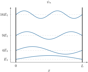
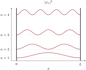
The levels and normalised eigenfunctions of a particle of mass $m$ in a box of length $L$ are

E_n = \frac{n^2h^2}{8mL^2}, \qquad \psi_n(x) = \sqrt{\frac2L}\,\sin\frac{n\pi x}{L}, \qquad n = 1, 2, 3, \dots

Proof. Inside, $\psi'' = -k^2\psi$ with $k^2 = 2mE/\hbar^2$ , so $\psi = A\sin kx + B\cos kx$ . Outside $\psi = 0$ and continuity gives $\psi(0) = 0$ , hence $B = 0$ , and $\psi(L) = 0$ , hence $\sin kL = 0$ with $A \ne 0$ : $kL = n\pi$ , $n$ a positive integer ( $n = 0$ gives $\psi = 0$ ; negative $n$ repeat the same functions). Then $E = \hbar^2k^2/2m = n^2\pi^2\hbar^2/2mL^2 = n^2h^2/8mL^2$ . Finally $\int_0^L A^2\sin^2(n\pi x/L)\,\dd x = A^2L/2 = 1$ gives $A = \sqrt{2/L}$ . ∎

Three features carry over to every bound system: the lowest energy is not zero (the particle can never be at rest), the levels spread apart as $n$ grows, and they crowd together as the box grows ( $E \propto 1/L^2$ ): a large box is nearly classical.

The first four levels of a particle in a box, each function drawn on its own level (dashed). Left: _n, with n - 1 nodes inside the box. Right: the probability density | _n|2. — The first four levels of a particle in a box, each function drawn on its own level (dashed). Left: $\psi_n$ , with $n - 1$ nodes inside the box. Right: the probability density $|\psi_n|^2$ .

Proposition 1.13 (The cubic box)

In a cubic box of side $L$ , $\psi = \psi_{n_x}(x)\psi_{n_y}(y)\psi_{n_z}(z)$ and $E = (n_x^2 + n_y^2 + n_z^2)\,h^2/8mL^2$ . Distinct triples with the same sum of squares give the same energy.

Proof. With $V = 0$ inside, $\hat H$ is a sum of three one-dimensional operators, one per coordinate. The product of three one-dimensional eigenfunctions is an eigenfunction of the sum, with the sum of the three eigenvalues; it vanishes on every face, as required. ∎

Definition 1.14 (Degenerate levels)

Linearly independent eigenfunctions with the same eigenvalue are degenerate levels; their number is the degeneracy $g$ of that energy.

Example 1.15 (Degeneracy and symmetry)

The level $n_x^2 + n_y^2 + n_z^2 = 6$ of the cube comes from $(2,1,1)$ , $(1,2,1)$ and $(1,1,2)$ : $g = 3$ . Stretch the box slightly along $z$ and the third function moves away from the other two: the degeneracy came from the symmetry of the cube. The same link between symmetry and degeneracy organises Chapters 4 and 5.

Conjugated dyes

In a symmetric cyanine dye, a chain of $j$ atoms joins the two nitrogens ( $j = 5$ , 7, 9 for the three dyes of the opening scene), and its $\pi$ electrons are delocalised along it. A chain of $j$ atoms carries $N = j + 1$ $\pi$ electrons: one per carbon, plus the lone pair of one nitrogen shared over the whole cation.

Proposition 1.16 (Free-electron absorption wavelength)

If $N$ $\pi$ electrons (an even number) fill the levels of a box of length $L$ , two per level, the longest-wavelength absorption, from the highest filled level $n = N/2$ to the next, is at

\lambda = \frac{8mcL^2}{h(N+1)}.

Proof. $\Delta E = E_{N/2+1} - E_{N/2} = [(N/2+1)^2 - (N/2)^2]\,h^2/8mL^2 = (N+1)\,h^2/8mL^2$ , and $\lambda = hc/\Delta E$ . ∎

Example 1.17 (The bare box fails, an extended box works)

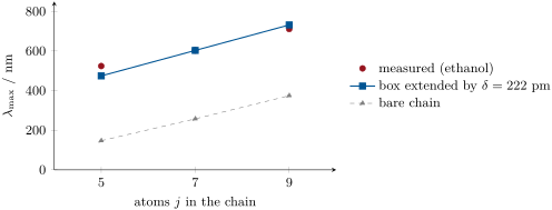
Take each bond of the chain equal to the C–C bond of benzene, $l = 139.7\,\mathrm{pm}$ , so that the bare chain measures $(j - 1)l$ . For the three dyes ( $N = 6$ , 8, 10) the formula gives 147, 257 and 374 nm, far below the measured maxima, 524, 603 and 711 nm in ethanol. The electrons are not stopped at the nitrogens: they spread into the rings. Extend the box by a length $\delta$ at each end and fit $\delta$ on the middle dye: $\delta = 222\,\mathrm{pm}$ , about one and a half bonds. The same $\delta$ then predicts 474 and 732 nm for the other two, within 10 % and 3 %. A single adjustable length explains a family of colours (figure below; the numbers are computed in the figure’s script).

Absorption maxima of the three cyanine dyes against the free-electron model: the bare chain, and the box extended by at each end, fitted on the middle dye. — Absorption maxima of the three cyanine dyes against the free-electron model: the bare chain, and the box extended by $\delta$ at each end, $\delta$ fitted on the middle dye.

In the lab — Measuring a dye series

The three dyes are weighed (a few milligrams), dissolved in ethanol and diluted until the absorbance at the maximum lies between 0.3 and 1. The spectrum of each is recorded between 400 and 800 nm in a 1 cm cuvette against a blank of pure ethanol, and $\lambda_{\max}$ read at the top of the main band. Cyanine dyes are stained and irritant solids: gloves, and weighing in a fume hood.

1.3 The harmonic oscillator

Near the bottom of any smooth potential well, $V \approx \frac12 k(x - x_e)^2$ : small vibrations of a bond, of an atom in a crystal, of a molecule in a cage are all approximately harmonic.

Definition 1.18 (Harmonic oscillator, force constant, reduced mass, zero-point energy)

A harmonic oscillator is a particle of mass $m$ in the potential $V = \frac12 kx^2$ ; $k$ is the force constant, and $\omega = \sqrt{k/m}$ its classical angular frequency. A diatomic molecule of atomic masses $m_1$ , $m_2$ vibrates as one particle of reduced mass $\mu = m_1m_2/(m_1 + m_2)$ in the potential of its bond. The energy of the lowest level of an oscillator is its zero-point energy.

Definition 1.19 (Ladder operators)

With $x_0 = \sqrt{\hbar/m\omega}$ , the ladder operators are

\hat a = \frac{1}{\sqrt2}\Big(\frac{\hat x}{x_0} + \frac{\iu x_0\hat p}{\hbar}\Big), \qquad \hat a^\dagger = \frac{1}{\sqrt2}\Big(\frac{\hat x}{x_0} - \frac{\iu x_0\hat p}{\hbar}\Big).

Theorem 1.20 (Levels of the harmonic oscillator)

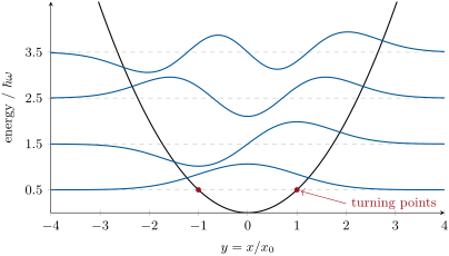
The levels of a harmonic oscillator are

E_v = \big(v + \tfrac12\big)\hbar\omega = \big(v + \tfrac12\big)h\nu, \qquad v = 0, 1, 2, \dots,

equally spaced by $h\nu$ , with the zero-point energy $\frac12h\nu$ .

Proof. From $[\hat x,\hat p] = \iu\hbar$ one computes $[\hat a,\hat a^\dagger] = 1$ and $\hat H = \hbar\omega(\hat a^\dagger\hat a + \frac12)$ . Write $\hat N = \hat a^\dagger\hat a$ . Then $[\hat N,\hat a] = -\hat a$ and $[\hat N,\hat a^\dagger] = \hat a^\dagger$ : if $\hat N\psi = \nu\psi$ , then $\hat N(\hat a\psi) = (\nu - 1)\hat a\psi$ and $\hat N(\hat a^\dagger\psi) = (\nu + 1)\hat a^\dagger\psi$ ; $\hat a$ lowers the eigenvalue by one, $\hat a^\dagger$ raises it. But $\nu = \langle\psi|\hat a^\dagger\hat a\psi\rangle/\langle\psi|\psi \rangle = \|\hat a\psi\|^2/\|\psi\|^2 \ge 0$ : the descent must stop, which happens only on a function with $\hat a\psi_0 = 0$ , of eigenvalue $\nu = 0$ . The eigenvalues of $\hat N$ are therefore $v = 0, 1, 2, \dots$ , and those of $\hat H$ are $(v + \frac12)\hbar\omega$ . ∎

Proposition 1.21 (The first wavefunctions)

In the reduced coordinate $y = x/x_0$ ,

\psi_0 \propto \eu^{-y^2/2}, \quad \psi_1 \propto 2y\,\eu^{-y^2/2}, \quad \psi_2 \propto (4y^2 - 2)\eu^{-y^2/2}, \quad \psi_3 \propto (8y^3 - 12y)\eu^{-y^2/2},

the Hermite polynomials times a Gaussian. $\psi_v$ is even for even $v$ , odd for odd $v$ .

Proof. $\hat a\psi_0 = 0$ reads $y\psi_0 + \dd\psi_0/\dd y = 0$ , whose solution is the Gaussian. Each next function is $\hat a^\dagger$ applied to the previous one, $\hat a^\dagger = \frac{1}{\sqrt2}(y - \dd/\dd y)$ , which multiplies the polynomial by $2y$ and subtracts its derivative: $1 \to 2y \to 4y^2 - 2 \to 8y^3 - 12y$ (up to factors). Changing $y$ into $-y$ changes the sign of $y$ and of $\dd/\dd y$ , so $\hat a^\dagger$ flips the parity at each step. ∎

The harmonic potential, its first four levels and wavefunctions, each drawn on its level. The wavefunctions reach beyond the classical turning points (y = ±1 for v = 0, red dots), where a classical particle would stop. — The harmonic potential, its first four levels and wavefunctions, each drawn on its level. The wavefunctions reach beyond the classical turning points ( $y = \pm1$ for $v = 0$ , red dots), where a classical particle would stop.

Example 1.22 (Zero-point energies of $\ce{H2}$ and $\ce{D2}$ )

The harmonic wavenumbers are $\tilde\omega_e = 4401.2\,\mathrm{cm}^{-1}$ for $\ce{H2}$ and $3115.5\,\mathrm{cm}^{-1}$ for $\ce{D2}$ , in the ratio $1.413$ , close to $\sqrt2$ : same bond and force constant, doubled reduced mass. The harmonic zero-point energies are half these, 2200.6 and $1557.8\,\mathrm{cm}^{-1}$ , $26.3\,\mathrm{kJ}/\mathrm{mol}$ and $18.6\,\mathrm{kJ}/\mathrm{mol}$ . A molecule can never lose this energy; the difference between isotopes is the source of the isotope effects of Chapters 11 and 12.

1.4 The rigid rotor

A diatomic molecule also turns about its centre of mass. Treated as two masses at a fixed distance $r$ , it is a rigid rotor of moment of inertia $I = \mu r^2$ , the reduced mass at distance $r$ from the axis.

Definition 1.23 (Rigid rotor, spherical harmonics)

A rigid rotor is a body of fixed shape turning freely; for a linear molecule, $\hat H = \hat L^2/2I$ , where $\hat L^2$ is the operator of the square of the angular momentum. Its eigenfunctions, which depend only on the angles $\theta$ and $\phi$ , are the spherical harmonics $Y_{l,m}(\theta,\phi)$ , labelled by $l = 0, 1, 2, \dots$ and $m = -l, \dots, l$ ; for a molecule $l$ is written $J$ .

The rotor on a ring (rotation in a plane, about a fixed axis) is solved first; it holds the essence.

Theorem 1.24 (The ring)

A particle of moment of inertia $I$ turning in a plane has levels $E_m = m^2\hbar^2/2I$ with $m = 0, \pm1, \pm2, \dots$ ; every level but $m = 0$ is doubly degenerate.

Proof. The only coordinate is the angle $\phi$ , and $\hat H = -(\hbar^2/2I)\, \dd^2/\dd\phi^2$ . The solutions of $\psi'' = -(2IE/\hbar^2)\psi$ are $\eu^{\iu m\phi}$ with $m^2 = 2IE/\hbar^2$ . A single-valued function must take the same value at $\phi$ and $\phi + 2\pi$ : $\eu^{2\pi\iu m} = 1$ , so $m$ is an integer. The functions with $m$ and $-m$ have the same energy and are independent. ∎

Theorem 1.25 (Levels of the rigid rotor)

$\hat L^2Y_{J,m} = J(J+1)\hbar^2\,Y_{J,m}$ and $\hat L_zY_{J,m} = m\hbar\, Y_{J,m}$ , so the levels of a linear rigid rotor are

E_J = \frac{\hbar^2}{2I}\,J(J+1), \qquad J = 0, 1, 2, \dots,

each with degeneracy $g_J = 2J + 1$ .

Proof. Admitted at this level. ∎

The general proof, by ladder operators for angular momentum, is treated in more advanced courses; here is a check. In spherical coordinates,

\hat L^2 = -\hbar^2\Big[\frac{1}{\sin\theta}\frac{\partial}{\partial\theta} \Big(\sin\theta\frac{\partial}{\partial\theta}\Big) + \frac{1}{\sin^2\theta}\frac{\partial^2}{\partial\phi^2}\Big].

For $Y_{1,0} \propto \cos\theta$ , the bracket is $\frac{1}{\sin\theta}(-2\sin\theta \cos\theta) = -2\cos\theta$ , so $\hat L^2Y_{1,0} = 2\hbar^2Y_{1,0} = 1(1+1)\hbar^2 Y_{1,0}$ . For $Y_{1,\pm1} \propto \sin\theta\,\eu^{\pm\iu\phi}$ the same computation gives $2\hbar^2$ again, and $\hat L_z = -\iu\hbar\,\partial/\partial \phi$ gives $\pm\hbar$ .

Proposition 1.26 (Real spherical harmonics)

For $l = 1$ , the combinations $Y_{1,0}$ , $(Y_{1,-1} - Y_{1,1})/\sqrt2$ and $\iu(Y_{1,-1} + Y_{1,1})/\sqrt2$ are real and proportional to $z/r$ , $x/r$ and $y/r$ ; for $l = 2$ the same construction gives functions proportional to $(3z^2 - r^2)$ , $xz$ , $yz$ , $xy$ and $x^2 - y^2$ , divided by $r^2$ .

Proof. $Y_{1,\pm1} \propto \mp\sin\theta\,\eu^{\pm\iu\phi}$ with the usual sign convention, so their difference over $\sqrt2$ is $\propto\sin\theta\cos\phi = x/r$ and the $\iu$ -weighted sum $\propto\sin\theta\sin\phi = y/r$ ; $\cos\theta = z/r$ . Each combination of degenerate eigenfunctions is still an eigenfunction of $\hat L^2$ (with the same $l$ ), though no longer of $\hat L_z$ . The $l = 2$ case is the same algebra with $\sin^2\theta\,\eu^{\pm2\iu\phi}$ and $\sin\theta\cos\theta\,\eu^{\pm\iu\phi}$ . ∎

These are the angular parts of the $p$ and $d$ orbitals drawn in the Year 2 volume: their names $p_x$ , $d_{xy}$ , $d_{z^2}$ are the Cartesian forms just found.

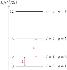
The first levels of a linear rigid rotor, E_J = J(J+1)\, 2/2I, with their degeneracies 2J + 1. The gaps grow as 2(J+1): the reason for the evenly spaced lines of . — The first levels of a linear rigid rotor, $E_J = J(J+1)\,\hbar^2/2I$ , with their degeneracies $2J + 1$ . The gaps grow as $2(J+1)$ : the reason for the evenly spaced lines of Chapter 6.

Example 1.27 (Rotational levels of $\ce{HCl}$ )

Spectroscopists write $E_J = hcB\,J(J+1)$ with the rotational constant $B = \hbar/(4\pi cI)$ in wavenumbers. For $\ce{H^{35}Cl}$ , $B = 10.593\,\mathrm{cm}^{-1}$ : the first levels lie at 0, 21.19, 63.56 and $127.12\,\mathrm{cm}^{-1}$ , all well below the thermal energy at room temperature, $kT/hc = 207\,\mathrm{cm}^{-1}$ . Many rotational levels are populated; only one vibrational level is ( $\tilde\omega_e = 2991\,\mathrm{cm}^{-1}$ ).

1.5 The hydrogen atom and tunnelling

The hydrogen atom, solved

An electron of charge $-e$ around a nucleus of charge $+e$ has $V = -e^2/ 4\pi\varepsilon_0r$ . With the reduced mass $\mu$ of electron and proton,

\hat H = -\frac{\hbar^2}{2\mu}\nabla^2 - \frac{e^2}{4\pi\varepsilon_0r},\qquad \nabla^2 = \frac{1}{r^2}\frac{\partial}{\partial r}\Big(r^2\frac{\partial}{ \partial r}\Big) - \frac{\hat L^2}{\hbar^2r^2}.

The angular part of $\nabla^2$ is the rotor operator: the solutions separate as $\psi = R(r)\,Y_{l,m}(\theta,\phi)$ , and $R$ obeys the radial equation

-\frac{\hbar^2}{2\mu}\frac{1}{r^2}\frac{\dd}{\dd r}\Big(r^2\frac{\dd R}{\dd r} \Big) + \Big[\frac{l(l+1)\hbar^2}{2\mu r^2} - \frac{e^2}{4\pi\varepsilon_0r} \Big]R = ER.

The rotation adds a centrifugal term $l(l+1)\hbar^2/2\mu r^2$ that keeps electrons with $l > 0$ away from the nucleus.

Theorem 1.28 (Levels of the hydrogen atom)

The bound levels of a hydrogen-like atom of nuclear charge $Ze$ are

E_n = -\frac{\mu}{m_e}\,\frac{Z^2hcR_\infty}{n^2}, \qquad n = 1, 2, \dots, \quad hcR_\infty = \frac{m_ee^4}{8\varepsilon_0^2h^2},

with $l = 0, \dots, n - 1$ ; the $1s$ and $2p$ radial functions are $R_{10} \propto \eu^{-Zr/a}$ and $R_{21} \propto r\,\eu^{-Zr/2a}$ , with $a = (m_e/\mu)a_0$ .

Partial proof. Take $Z = 1$ and try $R = \eu^{-r/a}$ with $l = 0$ . Then $R' = -R/a$ and $\frac{1}{r^2}(r^2R')' = R/a^2 - 2R/(ar)$ . The radial equation becomes $-\frac{\hbar^2}{2\mu}\big(\frac{1}{a^2} - \frac{2}{ar}\big) - \frac{e^2}{4\pi \varepsilon_0r} = E$ for all $r$ : the terms in $1/r$ cancel if $a = 4\pi\varepsilon_0\hbar^2/\mu e^2$ , and then $E = -\hbar^2/2\mu a^2 = -\mu e^4/8\varepsilon_0^2h^2$ , the $n = 1$ level. With $R = r\eu^{-r/b}$ and $l = 1$ , the same substitution leaves terms in $1/r^2$ (which cancel against the centrifugal term), in $1/r$ (which cancel if $b = 2a$ ) and a constant, $E = -\hbar^2/2\mu b^2$ , one quarter of the previous: the $n = 2$ level. The general case, a polynomial times $\eu^{-r/na}$ whose series must terminate to stay normalisable, is treated in more advanced courses. ∎

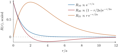
Radial functions of the hydrogen atom, from the solutions above (each scaled to a maximum near 1). R_20 has one radial node at r = 2a; R_21 vanishes at the nucleus, pushed out by the centrifugal term. — Radial functions of the hydrogen atom, from the solutions above (each scaled to a maximum near 1). $R_{20}$ has one radial node at $r = 2a$ ; $R_{21}$ vanishes at the nucleus, pushed out by the centrifugal term.

Example 1.29 (The ionisation energy of hydrogen)

$hcR_\infty = 13.6057\,\mathrm{eV}$ and $\mu/m_e = 1/(1 + m_e/m_p) = 0.999456$ , so $-E_1 = 13.598\,\mathrm{eV}$ : the measured ionisation energy of hydrogen, to the last digit given in the Year 1 volume. The reduced mass changes the fourth significant figure.

Tunnelling

Definition 1.30 (Tunnelling, transmission probability)

Tunnelling is the passage of a particle through a region where its energy is lower than the potential energy, forbidden in classical mechanics. The transmission probability $T$ of a barrier is the fraction of incident particles found beyond it.

Proposition 1.31 (Thin and thick barriers)

Inside a barrier of height $V_0 > E$ , $\psi$ is a combination of $\eu^{\pm\kappa x}$ with $\kappa = \sqrt{2m(V_0 - E)}/\hbar$ . For a rectangular barrier of width $a$ ,

T = \Big[1 + \frac{\sinh^2(\kappa a)}{4\varepsilon(1-\varepsilon)}\Big]^{-1}, \qquad \varepsilon = \frac{E}{V_0},

and for a thick barrier ( $\kappa a \gg 1$ ), $T \approx 16\varepsilon(1-\varepsilon) \,\eu^{-2\kappa a}$ .

Partial proof. In the barrier the Schrödinger equation reads $\psi'' = \kappa^2\psi$ , whose solutions are the two exponentials. Matching $\psi$ and $\psi'$ at the two walls with the waves $\eu^{\pm\iu kx}$ outside gives four linear equations; their solution, a page of algebra, is the formula for $T$ , which is admitted. For large $\kappa a$ , $\sinh\kappa a \approx \frac12\eu^{\kappa a}$ dominates and gives the thick-barrier form. ∎

The decisive factor is $\eu^{-2\kappa a}$ , and $\kappa \propto \sqrt m$ : tunnelling is a matter for the lightest particles, electrons first, then protons, and much less deuterons.

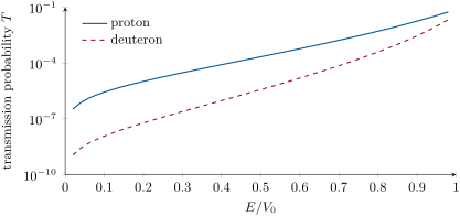
Transmission probability through a model barrier 0.40 eV high and 50 pm wide. At half the barrier height the proton passes about 58 times more often than the deuteron (log scale).

Remark 1.32 (Where tunnelling shows)

The ammonia molecule turns inside out, its nitrogen passing through the plane of the three hydrogens, by tunnelling through a low barrier; proton and hydrogen-atom transfers in enzymes show kinetic isotope effects far larger than Chapter 12 predicts without tunnelling; and the scanning tunnelling microscope images single atoms on a surface by the current of electrons tunnelling across a vacuum gap of a few tenths of a nanometre, a current that drops tenfold for each extra 0.1 nm.

History — Schrödinger, 1926

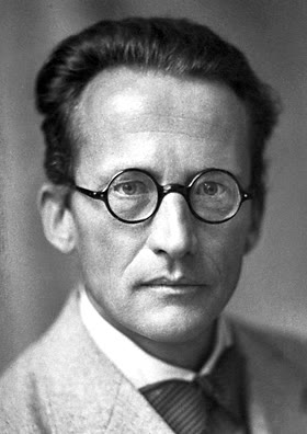
In four papers written in the first half of 1926, Erwin Schrödinger replaced the quantum rules of Bohr’s atom by a wave equation, solved it for the hydrogen atom, the oscillator and the rotor, and recovered the levels that spectroscopy had measured. The integers that Bohr had imposed by hand now appeared by themselves, as naturally as the number of nodes of a vibrating string. He shared the 1933 Nobel Prize in Physics with Paul Dirac.

1.6 Exercises

Exercise 1.1 ★

An electron is confined in a box of length (a) $1.00\,\mathrm{nm}$ , (b) $0.50\,\mathrm{nm}$ . Compute $E_1$ in joules and electronvolts, and the wavelength of the transition $n = 1 \to 2$ .

Solution

Solution of Exercise 1.1.

$E_1 = h^2/8m_eL^2$ . (a) $L = 1.00\,\mathrm{nm}$ : $E_1 = 6.02 \times 10^{-20}\,\mathrm{J} = 0.376\,\mathrm{eV}$ ; $\Delta E_{12} = 3E_1$ and $\lambda = hc/3E_1 = 1099\,\mathrm{nm}$ , in the near infrared. (b) $L = 0.50\,\mathrm{nm}$ : $E_1$ is four times larger, $2.41 \times 10^{-19}\,\mathrm{J}$ $= 1.50\,\mathrm{eV}$ , and $\lambda = 275\,\mathrm{nm}$ , in the ultraviolet.

Exercise 1.2 ★

List the five lowest levels of a particle in a cubic box, in units of $h^2/8mL^2$ , with their degeneracies.

Solution

Solution of Exercise 1.2.

$n_x^2 + n_y^2 + n_z^2 = 3$ (1,1,1): $g = 1$ ; $6$ (2,1,1 and permutations): $g = 3$ ; $9$ (2,2,1): $g = 3$ ; $11$ (3,1,1): $g = 3$ ; $12$ (2,2,2): $g = 1$ .

Exercise 1.3 ★

Compute the commutators $[\hat x^2,\hat p]$ and $[\hat p^2,\hat x]$ by acting on a function $f(x)$ .

Solution

Solution of Exercise 1.3.

$[\hat x^2,\hat p]f = -\iu\hbar x^2f' + \iu\hbar(x^2f)' = 2\iu\hbar xf$ , so $[\hat x^2,\hat p] = 2\iu\hbar\hat x$ . $[\hat p^2,\hat x]f = -\hbar^2[(xf)'' - xf''] = -2\hbar^2f'$ , so $[\hat p^2,\hat x] = -2\iu\hbar\hat p$ .

Exercise 1.4 ★

With $B = 10.593\,\mathrm{cm}^{-1}$ for $\ce{H^{35}Cl}$ , give the energies (in $\mathrm{cm}^{-1}$ ) and degeneracies of the levels $J = 0$ to 3, and the moment of inertia of the molecule.

Solution

Solution of Exercise 1.4.

$E_J/hc = BJ(J+1)$ : 0, 21.19, 63.56 and $127.12\,\mathrm{cm}^{-1}$ , with $g = 1$ , 3, 5, 7. $I = h/(8\pi^2cB) = 2.643 \times 10^{-47}\,\mathrm{kg}\,\mathrm{m}^{2}$ (with $c$ in $\mathrm{cm}/\mathrm{s}$ ).

Exercise 1.5 ★★

For the state $\psi_n$ of a particle in a box, compute $\langle x\rangle$ and $\langle x^2\rangle$ . Evaluate $\langle x^2\rangle$ for $n = 1$ and compare with the classical value $L^2/3$ for a particle equally likely to be anywhere.

Solution

Solution of Exercise 1.5.

$|\psi_n|^2$ is symmetric about $L/2$ , so $\langle x\rangle = L/2$ . With $\sin^2u = \frac12(1 - \cos2u)$ and two integrations by parts, $\langle x^2\rangle = L^2\big(\frac13 - \frac{1}{2n^2\pi^2}\big)$ . For $n = 1$ , $\langle x^2\rangle = 0.283L^2$ , less than the classical $L^2/3$ : the ground state piles up in the middle. As $n$ grows the classical value is recovered.

Exercise 1.6 ★★

Compute the harmonic zero-point energies of $\ce{H2}$ and $\ce{D2}$ in $\mathrm{kJ}/\mathrm{mol}$ from $\tilde\omega_e = 4401.2\,\mathrm{cm}^{-1}$ and $3115.5\,\mathrm{cm}^{-1}$ , and their difference. Which ratio of wavenumbers do you expect from the reduced masses, and how close is the measured one?

Solution

Solution of Exercise 1.6.

$1\,\mathrm{cm}^{-1} = 0.011\,963\,\mathrm{kJ}/\mathrm{mol}$ . ZPE( $\ce{H2}$ ) $= 2200.6 \times 0.011963 = 26.33\,\mathrm{kJ}/\mathrm{mol}$ , ZPE( $\ce{D2}$ ) $= 18.63\,\mathrm{kJ}/\mathrm{mol}$ ; difference $7.69\,\mathrm{kJ}/\mathrm{mol}$ . Same force constant, so $\tilde\omega \propto \mu^{-1/2}$ and the expected ratio is $\sqrt{\mu_D/\mu_H} = 1.4137$ (atomic masses 2.01410 and 1.00783); the measured ratio is 1.4127, within 0.07 % (the small difference comes from the electrons, which do not follow the nuclei perfectly).

Exercise 1.7 ★★

The function $\phi = Nx(L - x)$ is a rough guess for the ground state of the box. Normalise it, then compute its overlap $\langle\psi_1|\phi\rangle$ with the true ground state.

Solution

Solution of Exercise 1.7.

$\int_0^Lx^2(L - x)^2\,\dd x = L^5/30$ , so $N = \sqrt{30/L^5}$ . Then

\langle\psi_1|\phi\rangle = \sqrt{\tfrac2L}\sqrt{\tfrac{30}{L^5}}\int_0^Lx(L - x)\sin\tfrac{\pi x}{L}\,\dd x = \frac{\sqrt{60}}{L^3}\cdot\frac{4L^3}{\pi^3} = \frac{4\sqrt{60}}{\pi^3} = 0.99928 .

The parabola is 99.86 % ground state (the square of the overlap).

Exercise 1.8 ★★

Show that $\hat p = -\iu\hbar\,\dd/\dd x$ is Hermitian for functions that vanish at the ends of an interval, and that $\hat x\hat p$ is not.

Solution

Solution of Exercise 1.8.

$\langle f|\hat pg\rangle = -\iu\hbar\int f^*g'\,\dd x = -\iu\hbar[f^*g] + \iu\hbar\int f^{*\prime}g\,\dd x = \int(-\iu\hbar f')^*g\,\dd x = \langle\hat pf|g\rangle$ , the bracket vanishing at the ends. For $\hat x\hat p$ , using that $\hat x$ and $\hat p$ are each Hermitian: $\langle f|\hat x\hat pg\rangle = \langle\hat xf|\hat pg\rangle = \langle\hat p\hat xf|g\rangle$ , and $\hat p\hat x = \hat x\hat p - \iu\hbar \ne \hat x\hat p$ : not Hermitian (its symmetrised form $\frac12(\hat x\hat p + \hat p\hat x)$ is).

Exercise 1.9 ★★

Model hexa-1,3,5-triene as six $\pi$ electrons in a box of length $6l$ , $l = 139.7\,\mathrm{pm}$ (five bonds and half a bond at each end). Predict the wavelength of its first absorption. Is the molecule coloured?

Solution

Solution of Exercise 1.9.

$L = 6 \times 139.7 = 838\,\mathrm{pm}$ , $N = 6$ : $\lambda = 8m_ecL^2/(7h) = 331\,\mathrm{nm}$ . The absorption is in the ultraviolet: hexatriene is colourless.

Exercise 1.10 ★★★

For the model barrier of the figure ( $V_0 = 0.40\,\mathrm{eV}$ , $a = 50\,\mathrm{pm}$ ) at $E = V_0/2$ , compute $\kappa$ for a proton and a deuteron and, with the thick-barrier formula, the ratio $T_H/T_D$ . Compare with the exact ratio, 58.

Solution

Solution of Exercise 1.10.

$\kappa = \sqrt{2m(V_0 - E)}/\hbar$ with $V_0 - E = 0.20\,\mathrm{eV}$ : $\kappa_H = 9.82 \times 10^{10}\,\mathrm{m}^{-1}$ , $\kappa_D = 1.388 \times 10^{11}\,\mathrm{m}^{-1}$ . The prefactors cancel in the ratio: $T_H/T_D = \eu^{2a(\kappa_D - \kappa_H)} = \eu^{4.06} = 58$ , the exact value: the barrier is thick for both ( $\kappa a = 4.9$ and 6.9).

Exercise 1.11 ★★★

Treat the six $\pi$ electrons of benzene as particles on a ring of radius $139.7\,\mathrm{pm}$ (the C–C distance equals the radius of a regular hexagon). Fill the levels, then compute the wavelength of the transition from the highest filled to the lowest empty level.

Solution

Solution of Exercise 1.11.

Levels $E_m = m^2\hbar^2/2m_eR^2$ : $m = 0$ holds two electrons, $m = \pm1$ four. The highest filled is $|m| = 1$ , the lowest empty $|m| = 2$ : $\Delta E = 3\hbar^2/2m_eR^2 = 9.38 \times 10^{-19}\,\mathrm{J}$ , $\lambda = 212\,\mathrm{nm}$ , in the ultraviolet, as benzene’s strong absorption is.

Exercise 1.12 ★★★

For the hydrogen $1s$ state, $\psi = (\pi a^3)^{-1/2}\eu^{-r/a}$ . Compute the expectation value $\langle r\rangle$ and $\langle V\rangle$ , and check that $\langle V\rangle = 2E_1$ . (Use $\int_0^\infty r^n\eu^{-\beta r}\dd r = n!/\beta^{n+1}$ .)

Solution

Solution of Exercise 1.12.

$\langle r\rangle = \frac{4\pi}{\pi a^3}\int_0^\infty r^3\eu^{-2r/a}\dd r = \frac{4}{a^3}\cdot\frac{3!}{(2/a)^4} = \frac32a$ , $79.4\,\mathrm{pm}$ for $a = a_0$ . $\langle 1/r\rangle = \frac{4}{a^3}\cdot\frac{1!}{(2/a)^2} = \frac1a$ , so $\langle V\rangle = -e^2/(4\pi\varepsilon_0a)$ . Since $E_1 = -e^2/(8\pi\varepsilon_0a)$ (from $a = 4\pi\varepsilon_0\hbar^2/\mu e^2$ ), $\langle V\rangle = 2E_1$ , and the mean kinetic energy is $-E_1$ .

1.7 Problem: How Long Is a Dye?

Problem 1.1

Weekend problem — the free-electron model of three cyanine dyes: why a bare chain fails, which transitions are allowed, the energy scales of a molecule, and the box length that fits

Three symmetric cyanine dyes absorb at 524, 603 and 711 nm in ethanol; their conjugated chains, between and including the two nitrogens, have $j = 5$ , 7 and 9 atoms. Take each bond equal to $l = 139.7\,\mathrm{pm}$ , $m_e = 9.109 \times 10^{-31}\,\mathrm{kg}$ , $h = 6.626 \times 10^{-34}\,\mathrm{J}\,\mathrm{s}$ , $c = 2.998 \times 10^{8}\,\mathrm{m}/\mathrm{s}$ , $k = 1.381 \times 10^{-23}\,\mathrm{J}/\mathrm{K}$ , $1\,\mathrm{eV} = 1.602 \times 10^{-19}\,\mathrm{J}$ .

Part I — A bare chain.

Explain why a chain of $j$ atoms carries $N = j + 1$ $\pi$ electrons, and give $N$ for each dye.
Which levels of the box are the highest filled and the lowest empty for the first dye?
Show that the first absorption is at $\lambda = 8mcL^2/h(N+1)$ .
Give the bare length $L_0 = (j - 1)l$ of each chain.
Compute $\lambda$ for each dye with $L = L_0$ .
Compare with the measured values. In which direction is the model wrong, and what does that say about $L$ ?

Part II — Which transitions are allowed. The intensity of a transition $n \to n'$ is proportional to $|\langle \psi_n|x - L/2|\psi_{n'}\rangle|^2$ .

Show that $\psi_n$ is symmetric about the centre of the box for odd $n$ and antisymmetric for even $n$ .
Deduce that the integral vanishes when $n + n'$ is even.
Is the HOMO $\to$ LUMO transition of each dye allowed?
For the second dye, is the transition from the HOMO to the level above the LUMO allowed? From the level below the HOMO to the LUMO?
In the model, at what wavelength (as a fraction of the first one) would the next allowed transition from the HOMO lie?
Why does such a rule, derived from symmetry alone, survive the crudeness of the model?

Part III — The energy scales of a molecule.

Convert the absorption of the second dye into an energy in eV.
The vibration of $\ce{HCl}$ has $\tilde\omega_e = 2991\,\mathrm{cm}^{-1}$ : convert its quantum into eV.
The rotation of $\ce{HCl}$ has $B = 10.59\,\mathrm{cm}^{-1}$ : convert the gap between $J = 0$ and $J = 1$ into meV.
Compute $kT$ in meV at $298\,\mathrm{K}$ .
Which kinds of excitation are populated at room temperature?
In which regions of the spectrum are electronic, vibrational and rotational transitions observed?

Part IV — The box that fits.

From the measured 603 nm, compute the length $L$ the second dye’s box must have.
Writing $L = L_0 + 2\delta$ , deduce $\delta$ .
With this $\delta$ , predict $\lambda$ for the first dye; give the relative error.
Same question for the third dye.
Interpret $\delta$ : where do the $\pi$ electrons go beyond the nitrogens?
Express $\delta$ in bond lengths, and state the result of the problem: the effective extension of the box at each end.

Solution

Solution of Problem 1.1.

1. Each of the $j$ atoms gives one p orbital; the $j - 1$ carbons and one nitrogen give one electron each and the other nitrogen its lone pair, since the cation’s charge is spread over the chain: $N = j + 1$ , that is 6, 8 and 10. 2. Six electrons fill $n = 1$ , 2, 3: HOMO $n = 3$ , LUMO $n = 4$ . 3. $\Delta E = E_{N/2+1} - E_{N/2} = (N+1)h^2/8mL^2$ and $\lambda = hc/\Delta E = 8mcL^2/h(N+1)$ . 4. $L_0 = 4l$ , $6l$ , $8l$ : 559, 838 and $1118\,\mathrm{pm}$ . 5. 147, 257 and $374\,\mathrm{nm}$ . 6. All far too short (by factors 3.6, 2.3 and 1.9): the model’s box is too small, since $\lambda \propto L^2$ ; the electrons move over a longer distance than the chain between the nitrogens. 7. With the origin at the centre, $\psi_n \propto \cos(n\pi u/L)$ for odd $n$ and $\sin(n\pi u/L)$ for even $n$ ( $u = x - L/2$ ): even and odd functions of $u$ . 8. If $n + n'$ is even, $\psi_n$ and $\psi_{n'}$ have the same parity; their product times $u$ is odd and integrates to zero over a symmetric interval. 9. HOMO $N/2$ and LUMO $N/2 + 1$ have $n + n' = N + 1$ , odd: always allowed. 10. Second dye: HOMO 4, LUMO 5. $4 \to 6$ : sum even, forbidden. $3 \to 5$ : sum even, forbidden. 11. The next allowed one from $n = 4$ is $4 \to 7$ , with $\Delta E$ larger by $(49 - 16)/(25 - 16) = 3.67$ : at $\lambda/3.67$ , $164\,\mathrm{nm}$ for the second dye, deep in the ultraviolet. 12. It depends only on the symmetry of the potential about the chain’s centre, which the real symmetric dyes share. 13. $E = hc/\lambda = 3.294 \times 10^{-19}\,\mathrm{J} = 2.06\,\mathrm{eV}$ . 14. $hc\tilde\omega_e = 0.371\,\mathrm{eV}$ . 15. $2hcB = 4.21 \times 10^{-22}\,\mathrm{J} = 2.63\,\mathrm{meV}$ . 16. $kT = 25.7\,\mathrm{meV}$ . 17. Rotational levels only ( $2hcB \ll kT$ ); vibrational ( $15kT$ ) and electronic ( $80kT$ ) excitations are essentially not populated. 18. Electronic: visible and ultraviolet; vibrational: infrared; rotational: microwaves (and far infrared). 19. $L = \sqrt{\lambda h(N+1)/8mc}$ with $N = 8$ : $L = 1283\,\mathrm{pm}$ . 20. $\delta = (1283 - 838)/2 = 222\,\mathrm{pm}$ . 21. $L = 559 + 445 = 1003\,\mathrm{pm}$ , $\lambda = 474\,\mathrm{nm}$ , 9.5 % below 524 nm. 22. $L = 1118 + 445 = 1562\,\mathrm{pm}$ , $\lambda = 732\,\mathrm{nm}$ , 2.9 % above 711 nm. 23. Into the aromatic rings that carry the nitrogens: the $\pi$ system does not end at the nitrogen atoms, and the effective box includes part of each ring. 24. $\delta/l = 222/139.7 = 1.6$ : the box extends about $222\,\mathrm{pm}$ , a bond and a half, beyond each nitrogen, and with that one length the model reproduces the three colours within 10 %.

Terms defined in this chapter

See all 852 terms in the glossary