University Chemistry — Year 3 · Bachelor Year 3

12Theories of Reaction Rates

In 2017 a medicine was approved whose only difference from an older one is that the six hydrogen atoms of its two methoxy groups are deuterium atoms. The liver breaks the drug down by cutting exactly those C–H bonds, and a C–D bond is cut several times more slowly: the heavy molecule stays longer in the blood, and is taken in smaller, less frequent doses. Nothing in the Arrhenius law explains why a neutron in a nucleus should slow a reaction down. This chapter derives rate constants from molecular properties: first from collisions, then from the shape of the potential energy surface and the partition functions of the transition-state theory, which predicts the size of such isotope effects; it ends with reactions in solution, where the solvent sets a speed limit.

You already know

The Year 1 volume defined the rate constant, the Arrhenius law $k = A\eu^{-E_a/RT}$ with its activation energy and pre-exponential factor, elementary steps, the transition state, the energy profile along the reaction coordinate and the Hammond postulate. The Year 2 volume defined ionic strength and activity coefficients, with the Debye–Hückel limiting law $\log\gamma_i = -Az_i^2\sqrt I$ ( $A \approx 0.51$ in water at $25\,{}^{\circ}\mathrm{C}$ ), and fitted least-squares lines. Chapter 3 introduced potential energy surfaces; Chapters 10 and 11 computed equilibrium constants from partition functions and zero-point energies. From physics: the Maxwell–Boltzmann distribution of molecular speeds, and Fick’s law of diffusion.

Medicines on a pharmacy shelf. Replacing hydrogen by deuterium at the bonds the liver attacks first can lengthen the time a drug stays in the body.

12.1 Collision theory

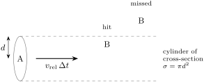
Two molecules in a gas can react only if they meet. Model them as hard spheres of diameters $d_{\mathrm A}$ and $d_{\mathrm B}$ : they collide when their centres pass within $d = \frac12(d_{\mathrm A} + d_{\mathrm B})$ of each other.

Definition 12.1 (Collision cross-section, steric factor)

The collision cross-section of two molecules is the area $\sigma = \pi d^2$ of the disc, perpendicular to their relative velocity, inside which the centre of one must pass for it to hit the other. The steric factor $P$ is the ratio of the measured pre-exponential factor of a reaction to the one predicted by collision theory.

The collision cylinder. Moving at the relative speed v_ rel, molecule A sweeps in a time t a cylinder of cross-section = π d2, with d the sum of the two radii; every B whose centre lies inside is hit. — The collision cylinder. Moving at the relative speed $v_{\mathrm{rel}}$ , molecule A sweeps in a time $\Delta t$ a cylinder of cross-section $\sigma = \pi d^2$ , with $d$ the sum of the two radii; every B whose centre lies inside is hit.

Theorem 12.2 (Collision-theory rate constant)

If every collision whose kinetic energy along the line of centres exceeds a threshold $E_0$ (per mole) leads to reaction, the rate constant of $\mathrm{A + B} \to$ products is

k = \sigma\bar v_{\mathrm{rel}}N_A\,\eu^{-E_0/RT}, \qquad \bar v_{\mathrm{rel}} = \sqrt{\frac{8kT}{\pi\mu}},\ \mu = \frac{m_{\mathrm A}m_{\mathrm B}}{m_{\mathrm A} + m_{\mathrm B}} .

Partial proof. In a time $\Delta t$ a molecule A sweeps a volume $\sigma v_{\mathrm{rel}}\Delta t$ and hits the $n_{\mathrm B}\sigma v_{\mathrm{rel}}\Delta t$ molecules B it contains: the collision rate per unit volume is $\sigma\bar v_{\mathrm{rel}}n_{\mathrm A}n_{\mathrm B}$ , with $\bar v_{\mathrm{rel}}$ the mean relative speed given by the Maxwell–Boltzmann distribution (admitted from physics, with the reduced mass). Weighting each collision by its speed and keeping those whose energy along the line of centres exceeds the threshold leaves the fraction $\eu^{-E_0/RT}$ of the collision rate (the integration over the impact parameter is admitted). Converting number densities into molar concentrations multiplies by $N_A$ . ∎

Since $\bar v_{\mathrm{rel}} \propto \sqrt T$ , the activation energy $E_a = RT^2\,\dd\ln k/\dd T$ is $E_0 + \frac12RT$ , close to the threshold. The pre-exponential factor is of the order of $10^{11}$ $\mathrm{L}\,\mathrm{mol}^{-1}\,\mathrm{s}^{-1}$ for small molecules. Measured factors are often much smaller: $P \ll 1$ for molecules that must meet in a particular orientation, and the cross-section has no unique value for real molecules, which are not hard spheres. Collision theory gives the order of magnitude and the temperature dependence; it cannot give $E_0$ , which needs the potential energy surface.

12.2 Potential energy surfaces

The reaction $\mathrm{H_A + H_BH_C \to H_AH_B + H_C}$ is the simplest there is. For a collinear approach the energy depends on two distances, $r_{\mathrm{AB}}$ and $r_{\mathrm{BC}}$ , and can be drawn as a map.

Definition 12.3 (Saddle point, minimum energy path)

A saddle point of a potential energy surface is a point where the gradient vanishes, the energy is a maximum along one direction and a minimum along all others. The minimum energy path is the path of steepest descent from the saddle point to the reactant and product valleys; its length measured along it is the reaction coordinate, and the saddle point is the transition state.

A model potential energy surface for collinear H + H2 (LEPS form built from the Morse curve of H2, with a Sato parameter of 0.17 chosen as a model constant). Contours from -4.65\, eV to -0.8\, eV, energy zero for three separate atoms; the valleys lie at -4.75\, eV, the depth of the H2 well. Dashed: the minimum energy path, which crosses the symmetric saddle at r_ AB = r_ BC = 0.92\, Å, 0.27\, eV above the valleys in this model. — A model potential energy surface for collinear $\ce{H + H2}$ (LEPS form built from the Morse curve of $\ce{H2}$ , with a Sato parameter of 0.17 chosen as a model constant). Contours from $-4.65\,\mathrm{eV}$ to $-0.8\,\mathrm{eV}$ , energy zero for three separate atoms; the valleys lie at $-4.75\,\mathrm{eV}$ , the depth of the $\ce{H2}$ well. Dashed: the minimum energy path, which crosses the symmetric saddle at $r_{\mathrm{AB}} = r_{\mathrm{BC}} = 0.92\,\text{Å}$ , $0.27\,\mathrm{eV}$ above the valleys in this model.

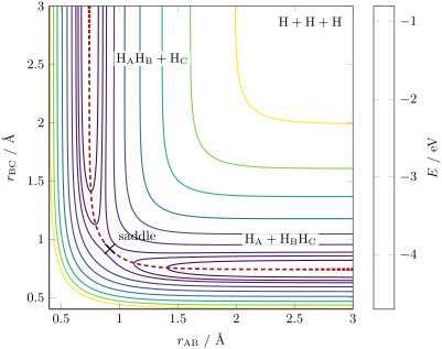
The path climbs out of the reactant valley, where $r_{\mathrm{BC}}$ stays near the $\ce{H2}$ bond length while A approaches, crosses the saddle, and descends into the product valley. At the saddle both bonds are stretched to $0.92\,\text{Å}$ : the old bond is half broken and the new one half made, and the energy cost of this compromise is the barrier. For the symmetric reaction the saddle lies on the diagonal; for an exothermic reaction it moves towards the reactant valley (an early barrier, a reactant-like transition state, as the Hammond postulate says), for an endothermic one towards the product valley (a late barrier). The position decides which energy helps: translational energy, directed along the entrance valley, carries the molecules over an early barrier; a late barrier, around a corner, is crossed more easily with vibrational energy in the breaking bond. These are Polanyi’s rules, confirmed by molecular-beam experiments.

12.3 Transition-state theory

Definition 12.4 (Activated complex)

The activated complex of an elementary step is the set of configurations of the reacting system in a thin slice around the saddle point, perpendicular to the minimum energy path; it is treated as a species $\ce{AB^{\ddagger}}$ , with its own partition function.

Definition 12.5 (Transition-state theory, transmission coefficient)

Transition-state theory assumes that the activated complexes are in equilibrium with the reactants, that every complex crossing the saddle region towards the products goes on to form them, and that the motion along the reaction coordinate is a free translation. The transmission coefficient $\kappa \le 1$ corrects for the complexes that recross back to the reactants.

Theorem 12.6 (Eyring equation)

For an elementary step $\mathrm{A + B} \to \mathrm{AB}^{\ddagger} \to$ products,

k = \kappa\frac{k_BT}{h}\overline{K}{}^{\ddagger}, \qquad \overline{K}{}^{\ddagger} = \frac{\bar q^{\ddagger}/N_A}{(q_{\mathrm A}/N_A)(q_{\mathrm B}/N_A)}\,\eu^{-\Delta E_0^{\ddagger}/RT},

where $\bar q^{\ddagger}$ is the partition function of the activated complex with the reaction-coordinate motion removed, $q$ are molar partition functions per unit volume, and $\Delta E_0^{\ddagger}$ is the height of the zero-point level of the complex above that of the reactants. In thermodynamic form, with $c^\circ = 1\,\mathrm{mol}/\mathrm{L}$ and the molecularity $m$ ,

k = \kappa\frac{k_BT}{h}(c^\circ)^{1-m}\,\eu^{\Delta^{\ddagger}S^\circ/R}\,\eu^{-\Delta^{\ddagger}H^\circ/RT}.

This statement is the Eyring equation; $k_B$ is the Boltzmann constant, written so to avoid confusion with $k$ .

Proof. Quasi-equilibrium: $[\ce{AB^{\ddagger}}] = K^{\ddagger}[\mathrm A][\mathrm B]$ , with $K^{\ddagger}$ from the partition functions (Theorem 11.10, written with concentrations). Of the vibrations of the complex, one is the motion along the reaction coordinate: a very loose vibration of frequency $\nu \ll k_BT/h$ , whose partition function is $k_BT/h\nu$ (the high-temperature limit of Proposition 10.16); hence $q^{\ddagger} = \bar q^{\ddagger}k_BT/h\nu$ . The complexes cross towards the products at the frequency $\nu$ of this motion, so the rate is $\nu[\ce{AB^{\ddagger}}] = \nu\frac{k_BT}{h\nu}\overline{K}{}^{\ddagger}[\mathrm A][\mathrm B]$ : the unknown $\nu$ cancels. Writing $\overline{K}{}^{\ddagger} = (c^\circ)^{1-m}\eu^{-\Delta^{\ddagger}G^\circ/RT}$ and $\Delta^{\ddagger}G^\circ = \Delta^{\ddagger}H^\circ - T\Delta^{\ddagger}S^\circ$ gives the second form, with $\kappa$ inserted for recrossing. ∎

The factor $k_BT/h$ is $6.2 \times 10^{12}\,\mathrm{s}^{-1}$ at $298\,\mathrm{K}$ : the rate of a unimolecular step with no barrier and no entropy loss. Everything specific to the reaction lies in the quantities of activation.

Definition 12.7 (Gibbs energy, enthalpy and entropy of activation)

The Gibbs energy of activation $\Delta^{\ddagger}G^\circ$ , enthalpy of activation $\Delta^{\ddagger}H^\circ$ and entropy of activation $\Delta^{\ddagger}S^\circ$ of an elementary step are the standard Gibbs energy, enthalpy and entropy of formation of the activated complex (without its reaction-coordinate motion) from the reactants, defined by the Eyring equation.

Proposition 12.8 (Activation energy and enthalpy of activation)

For a reaction in solution, $E_a = \Delta^{\ddagger}H^\circ + RT$ ; for a bimolecular gas reaction, $E_a = \Delta^{\ddagger}H^\circ + 2RT$ .

Proof. $E_a = RT^2\,\dd\ln k/\dd T$ , and $\ln k = \ln T + \Delta^{\ddagger}S^\circ/R - \Delta^{\ddagger}H^\circ/RT +$ const: $E_a = RT + \Delta^{\ddagger}H^\circ$ when the activation parameters do not vary with $T$ . In solution this is the result. In the gas phase the van ’t Hoff relation for $K^{\ddagger}$ written in concentrations involves the internal energy, $\Delta^{\ddagger}U^\circ = \Delta^{\ddagger}H^\circ - \Delta n^{\ddagger}RT$ with $\Delta n^{\ddagger} = 1 - m$ : for $m = 2$ , $E_a = \Delta^{\ddagger}H^\circ + 2RT$ . ∎

The entropy of activation reads the structure of the transition state. Two molecules that combine into one complex lose translational and rotational freedom: $\Delta^{\ddagger}S^\circ$ is strongly negative, $-50$ to $-150$ $\mathrm{J}\,\mathrm{K}^{-1}\,\mathrm{mol}^{-1}$ , for associative steps and cyclic transition states. A molecule that loosens a bond on its way to dissociating gains freedom: $\Delta^{\ddagger}S^\circ > 0$ .

Proposition 12.9 (Standard errors of a fitted line)

For a least-squares line $y = a + bx$ through $n$ points whose $y$ carry independent errors of the same variance, estimated by $s^2 = \sum_i(y_i - a - bx_i)^2/(n - 2)$ , the slope and intercept have the standard errors

s_b = \frac{s}{\sqrt{\sum_i(x_i - \bar x)^2}}, \qquad s_a = s\sqrt{\frac1n + \frac{\bar x^2}{\sum_i(x_i - \bar x)^2}} .

Proof. $b = \sum_i(x_i - \bar x)y_i/S_{xx}$ , with $S_{xx} = \sum_i(x_i - \bar x)^2$ , is a linear combination of independent $y_i$ of variance $\sigma^2$ : its variance is $\sigma^2\sum_i(x_i - \bar x)^2/S_{xx}^2 = \sigma^2/S_{xx}$ . Likewise $a = \bar y - b\bar x$ , and $\bar y$ and $b$ are uncorrelated (their covariance is $\sigma^2\sum_i(x_i - \bar x)/(nS_{xx}) = 0$ ), so $\operatorname{var}a = \sigma^2/n + \bar x^2\sigma^2/S_{xx}$ . Replacing $\sigma^2$ by its estimate $s^2$ (the divisor $n - 2$ accounts for the two fitted parameters, admitted) gives the result. ∎

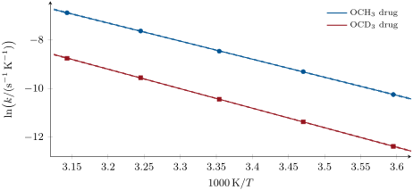
Method 12.10 (An Eyring plot with uncertainties)

Measure $k$ at five or more temperatures spread over 30 to $40\,\mathrm{K}$ .
Plot $y = \ln(k/T)$ against $x = 1/T$ and fit the least-squares line $y = a + bx$ .
$\Delta^{\ddagger}H^\circ = -Rb$ and $\Delta^{\ddagger}S^\circ = R[a - \ln(k_B/h)]$ ( $\ln(k_B/h) = 23.760$ with $k$ in $\mathrm{s}^{-1}$ ).
Their standard errors are $Rs_b$ and $Rs_a$ ; a 95 % confidence interval multiplies them by Student’s $t$ for $n - 2$ degrees of freedom (3.18 for five points).
The intercept lies far outside the measured range, at $1/T = 0$ : $\Delta^{\ddagger}S^\circ$ is always much less precise than $\Delta^{\ddagger}H^\circ$ , and the two errors are correlated.

Eyring plots of the weekend problem’s rate constants (data of the problem) for the drug and its deuterated analogue, with the least-squares lines and their 95 % confidence bands (dashed, hardly wider than the lines: the points scatter by about 1 %). The lines are parallel within their uncertainty: the same entropy of activation, enthalpies of activation that differ by about 5\, kJ/ mol. — Eyring plots of the weekend problem’s rate constants (data of the problem) for the drug and its deuterated analogue, with the least-squares lines and their 95 % confidence bands (dashed, hardly wider than the lines: the points scatter by about 1 %). The lines are parallel within their uncertainty: the same entropy of activation, enthalpies of activation that differ by about $5\,\mathrm{kJ}/\mathrm{mol}$ .

12.4 Kinetic isotope effects

Definition 12.11 (Kinetic isotope effects)

The kinetic isotope effect of a step is the ratio $k_{\mathrm{light}}/k_{\mathrm{heavy}}$ of its rate constants for two isotopologues, most often $k_{\mathrm H}/k_{\mathrm D}$ . It is a primary kinetic isotope effect when the bond to the substituted atom is made or broken in the step, a secondary kinetic isotope effect when it is not.

Proposition 12.12 (Maximum primary kinetic isotope effect)

If the stretching vibration of an X–H bond becomes the reaction coordinate, so that its zero-point energy is lost in the transition state while all other contributions are the same for H and D,

\frac{k_{\mathrm H}}{k_{\mathrm D}} = \exp\Bigl[\frac{hc(\tilde\nu_{\mathrm{XH}} - \tilde\nu_{\mathrm{XD}})}{2k_BT}\Bigr], \qquad \frac{\tilde\nu_{\mathrm{XH}}}{\tilde\nu_{\mathrm{XD}}} = \sqrt{\frac{\mu_{\mathrm{XD}}}{\mu_{\mathrm{XH}}}} .

Proof. The potential energy surface is the same for both isotopologues (the electrons do not see the neutron). In the reactant the X–H stretch holds $\frac12hc\tilde\nu_{\mathrm{XH}}$ of zero-point energy; in the transition state this mode has become the reaction coordinate and holds none. The barrier measured between zero-point levels is therefore lower for H by $\frac12hc\tilde\nu_{\mathrm{XH}}$ and for D by $\frac12hc\tilde\nu_{\mathrm{XD}}$ : $\Delta E_0^{\ddagger}(\mathrm D) - \Delta E_0^{\ddagger}(\mathrm H) = \frac12hc(\tilde\nu_{\mathrm{XH}} - \tilde\nu_{\mathrm{XD}})$ , and the Eyring equation gives the ratio when the other factors cancel. The wavenumber of a stretch is proportional to $1/\sqrt\mu$ (Chapter 6). ∎

Origin of the primary kinetic isotope effect. In the reactant, the C–H stretch holds more zero-point energy than the C–D stretch (levels above the bottom of the well, dashed); in the transition state this vibration has become the reaction coordinate, and both isotopologues reach the same top. The barrier is larger for D by the difference of the zero-point energies.

Maximum primary kinetic isotope effect against temperature for the loss of a C–H, N–H or O–H stretch (fundamentals of CH4, NH3 and H2O; the deuterium wavenumbers from the reduced masses). At 298\, K it is 6.5 for C–H; it decreases towards 1 as the temperature rises. — Maximum primary kinetic isotope effect against temperature for the loss of a C–H, N–H or O–H stretch (fundamentals of $\ce{CH4}$ , $\ce{NH3}$ and $\ce{H2O}$ ; the deuterium wavenumbers from the reduced masses). At $298\,\mathrm{K}$ it is 6.5 for C–H; it decreases towards 1 as the temperature rises.

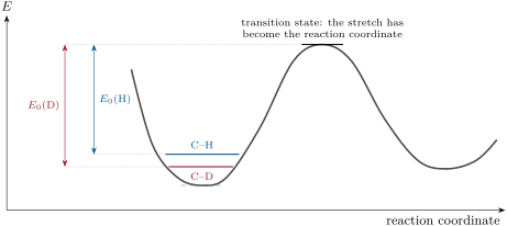
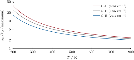
The maximum C–H value at room temperature, about 7, is a benchmark. Observed effects of 2 to 7 indicate that the C–H bond is broken in the rate-determining step; smaller values that the transition state keeps part of the stretch (asymmetric, early or late hydrogen transfers), or that the step is not the slowest. Values much larger than 7 at room temperature cannot come from zero-point energies: they reveal tunnelling (Chapter 1), which a particle of twice the mass does much less. Secondary effects, from changes of the bending vibrations of C–H bonds next to the reacting centre, are small, typically 0.8 to 1.2 per deuterium; they distinguish, for example, a carbon that becomes trigonal (sp $^3$ to sp $^2$ , $k_{\mathrm H}/k_{\mathrm D} > 1$ ) from one that becomes tetrahedral ( $< 1$ ).

Method 12.13 (Measuring a kinetic isotope effect by competition)

Run the reaction on a mixture of the two isotopologues, or on a molecule carrying H on one site and D on an equivalent one.
Stop at low conversion and measure the ratio of the H and D products by mass spectrometry or NMR.
The product ratio, corrected for the starting ratio, is $k_{\mathrm H}/k_{\mathrm D}$ ; both isotopologues see exactly the same conditions, which makes the method more precise than two separate rate measurements.

12.5 Reactions in solution

In a liquid a molecule does not fly freely between collisions: it rattles in a cage of neighbours, colliding with them many times before it diffuses away. Two reactants that meet stay together for many collisions, an encounter.

Definition 12.14 (Diffusion and activation control, cage effect)

A reaction in solution is diffusion-controlled when reaction at every encounter is fast, so that its rate is the rate at which the reactants diffuse together; it is activation-controlled when only a small fraction of encounters lead to reaction. The cage effect is the confinement of a pair of molecules by the surrounding solvent, which makes them collide repeatedly during one encounter.

Proposition 12.15 (Smoluchowski limit)

The rate constant of a diffusion-controlled reaction between spheres that react at the distance $R^*$ is $k_d = 4\pi N_A(D_{\mathrm A} + D_{\mathrm B})R^*$ . With the Stokes–Einstein relation $D = k_BT/6\pi\eta a$ for spheres of radius $a$ in a solvent of viscosity $\eta$ , and $R^* = a_{\mathrm A} + a_{\mathrm B}$ with $a_{\mathrm A} = a_{\mathrm B}$ ,

k_d = \frac{8RT}{3\eta} .

Partial proof. Fix A at the origin; B diffuses with the relative diffusion coefficient $D = D_{\mathrm A} + D_{\mathrm B}$ and is destroyed at $r = R^*$ . In the steady state the radial flux through every sphere is the same, $J = 4\pi r^2D\,\dd c/\dd r$ (Fick’s law, from physics); integrating from $R^*$ , where $c = 0$ , to infinity, where $c = c_{\mathrm B}$ , gives $J = 4\pi DR^*c_{\mathrm B}$ , the rate per molecule A. With Stokes–Einstein (admitted), $(D_{\mathrm A} + D_{\mathrm B})R^* = \frac{k_BT}{6\pi\eta}(\frac{1}{a} + \frac1a)(2a) = \frac{2k_BT}{3\pi\eta}$ , and $k_d = 4\pi N_A \times \frac{2k_BT}{3\pi\eta} = 8RT/3\eta$ . ∎

Example 12.16 (Speed limits in water and in hexane)

At $298.15\,\mathrm{K}$ , water ( $\eta = 0.890\,\mathrm{mPa}\,\mathrm{s}$ ) gives $k_d = 8 \times 8.314 \times 298.15/(3 \times 0.890 \times 10^{-3}) = 7.4 \times 10^{6}\,\mathrm{m}^{3}\,\mathrm{mol}^{-1}\,\mathrm{s}^{-1} = 7.4 \times 10^{9}\,\mathrm{L}\,\mathrm{mol}^{-1}\,\mathrm{s}^{-1}$ ; hexane ( $\eta = 0.298\,\mathrm{mPa}\,\mathrm{s}$ ), $2.2 \times 10^{10}\,\mathrm{L}\,\mathrm{mol}^{-1}\,\mathrm{s}^{-1}$ . No bimolecular reaction between neutral molecules of ordinary size is faster; measured constants near these values (the quenching of excited states, the recombination of radicals) are diffusion-controlled. Ions of opposite charge attract and can go faster.

Ions in solution add an electrostatic contribution to the activation: the transition state of two ions has charge $z_{\mathrm A} + z_{\mathrm B}$ , and its activity coefficient differs from the product of theirs.

Definition 12.17 (Kinetic salt effect)

The kinetic salt effect is the change of the rate constant of a reaction between ions with the ionic strength of the solution.

Proposition 12.18 (Brønsted–Bjerrum equation)

For a step between ions of charges $z_{\mathrm A}$ and $z_{\mathrm B}$ in dilute aqueous solution,

\log k = \log k_0 + 2Az_{\mathrm A}z_{\mathrm B}\sqrt I,

where $k_0$ is the rate constant at zero ionic strength.

Proof. In transition-state theory the equilibrium with the activated complex is written with activities: $[\ce{AB^{\ddagger}}] = K^{\ddagger}[\mathrm A][\mathrm B]\gamma_{\mathrm A}\gamma_{\mathrm B}/\gamma^{\ddagger}$ , so $k = k_0\gamma_{\mathrm A}\gamma_{\mathrm B}/\gamma^{\ddagger}$ . With the limiting law: $\log(\gamma_{\mathrm A}\gamma_{\mathrm B}/\gamma^{\ddagger}) = -A\sqrt I[z_{\mathrm A}^2 + z_{\mathrm B}^2 - (z_{\mathrm A} + z_{\mathrm B})^2] = 2Az_{\mathrm A}z_{\mathrm B}\sqrt I$ . ∎

Ions of the same sign react faster when salt is added (the ionic atmosphere screens their repulsion), ions of opposite signs more slowly, and a neutral reactant shows no primary salt effect: a plot of $\log k$ against $\sqrt I$ at low ionic strength measures the product of the charges of the reacting species.

Method 12.19 (What activation parameters say about a mechanism)

$\Delta^{\ddagger}S^\circ$ strongly negative: an associative step, an ordered or cyclic transition state, or one that orders the solvent (charge creation); positive: a dissociative step.
A primary $k_{\mathrm H}/k_{\mathrm D}$ of 2 to 7: the bond to H is broken in the rate-determining step; above about 10 at room temperature: tunnelling.
The slope of $\log k$ against $\sqrt I$ : the product $z_{\mathrm A}z_{\mathrm B}$ of the charges that meet in the rate-determining step.
A rate constant near $10^{10}$ $\mathrm{L}\,\mathrm{mol}^{-1}\,\mathrm{s}^{-1}$ that varies as $T/\eta$ : diffusion control.

In the lab — A jacketed cell for an Eyring study

The reaction is followed by its absorbance in a spectrophotometer cell whose jacket is fed by a thermostated bath; a thermocouple in a reference cell checks the temperature to $0.1\,\mathrm{K}$ . Five to seven temperatures, each measured in triplicate, give an Eyring plot; the solutions are equilibrated in the holder before mixing, since a reaction started at the wrong temperature biases the first points.

History — Eyring, Evans and Polanyi, 1935

In 1935 Henry Eyring, in Princeton, and Meredith Gwynne Evans and Michael Polanyi, in Manchester, published independently the theory of the activated complex. Eyring had computed, with Polanyi in Berlin in 1931, the first potential energy surface for $\ce{H + H2}$ , by a semi-empirical method of the kind used for the figure of this chapter. The theory was received with suspicion: a journal first rejected Eyring’s paper as unsound, and it was published only after other physicists vouched for it.

12.6 Exercises

Exercise 12.1 ★

For $\ce{NO + O3 -> NO2 + O2}$ take $\sigma = 0.43\,\mathrm{nm}^{2}$ (data of the exercise). Compute $\bar v_{\mathrm{rel}}$ at $298\,\mathrm{K}$ ( $\mu = 18.46\,\mathrm{u}$ ), the collision-theory pre-exponential factor, and the steric factor given the measured $A = 2.07 \times 10^{-12}\,\mathrm{cm}^{3}\,\mathrm{s}^{-1}$ per molecule.

Solution

Solution of Exercise 12.1.

$\bar v_{\mathrm{rel}} = \sqrt{8 \times 1.381\times10^{-23} \times 298/(\pi \times 18.46 \times 1.661\times10^{-27})} = 585\,\mathrm{m}/\mathrm{s}$ . $\sigma\bar v_{\mathrm{rel}}N_A = 0.43\times10^{-18} \times 585 \times 6.022\times10^{23} = 1.51 \times 10^{8}\,\mathrm{m}^{3}\,\mathrm{mol}^{-1}\,\mathrm{s}^{-1} = 1.5 \times 10^{11}\,\mathrm{L}\,\mathrm{mol}^{-1}\,\mathrm{s}^{-1}$ . Measured: $2.07\times10^{-12} \times 6.022\times10^{23}\times10^{-3} = 1.25 \times 10^{9}\,\mathrm{L}\,\mathrm{mol}^{-1}\,\mathrm{s}^{-1}$ , so $P = 0.008$ : fewer than one collision in a hundred has the right orientation (the O of NO must meet a terminal O of $\ce{O3}$ ).

Exercise 12.2 ★

A reaction in solution has $E_a = 75.0\,\mathrm{kJ}/\mathrm{mol}$ near $298\,\mathrm{K}$ . What is $\Delta^{\ddagger}H^\circ$ ? And for a bimolecular gas reaction with the same $E_a$ ?

Solution

Solution of Exercise 12.2.

$\Delta^{\ddagger}H^\circ = 75.0 - 2.48 = 72.5\,\mathrm{kJ}/\mathrm{mol}$ in solution; $75.0 - 4.96 = 70.0\,\mathrm{kJ}/\mathrm{mol}$ for a bimolecular gas reaction.

Exercise 12.3 ★

Predict the sign of $\Delta^{\ddagger}S^\circ$ for: a Diels–Alder cycloaddition; the unimolecular loss of $\ce{N2}$ from an azo compound; an $\mathrm{S_N2}$ reaction between two neutral molecules that creates two ions in a polar solvent.

Solution

Solution of Exercise 12.3.

Diels–Alder: strongly negative (two molecules form one cyclic complex). Loss of $\ce{N2}$ : positive (a bond loosens, freedom is gained). Ions created in a polar solvent: negative, the developing charges order the solvent around them.

Exercise 12.4 ★

Compute the diffusion-controlled rate constant in water and in hexane at $298.15\,\mathrm{K}$ . Which solvent allows faster encounters, and why?

Solution

Solution of Exercise 12.4.

Water: $8 \times 8.314 \times 298.15/(3 \times 0.890 \times 10^{-3}) = 7.4 \times 10^{9}\,\mathrm{L}\,\mathrm{mol}^{-1}\,\mathrm{s}^{-1}$ ; hexane $2.2 \times 10^{10}\,\mathrm{L}\,\mathrm{mol}^{-1}\,\mathrm{s}^{-1}$ . Hexane, three times less viscous: molecules diffuse three times faster.

Exercise 12.5 ★★

A first-order reaction has $k = 1.00 \times 10^{-3}\,\mathrm{s}^{-1}$ at $298.15\,\mathrm{K}$ and $1.00 \times 10^{-2}\,\mathrm{s}^{-1}$ at $318.15\,\mathrm{K}$ . Compute $\Delta^{\ddagger}H^\circ$ and $\Delta^{\ddagger}S^\circ$ , and $E_a$ for comparison.

Solution

Solution of Exercise 12.5.

$\ln(k_2T_1/k_1T_2) = \ln(10 \times 298.15/318.15) = 2.238$ ; $\Delta^{\ddagger}H^\circ = 8.3145 \times 2.238/(1/298.15 - 1/318.15) = 88.2\,\mathrm{kJ}/\mathrm{mol}$ . $\Delta^{\ddagger}S^\circ = R[\ln(kh/k_BT) + \Delta^{\ddagger}H^\circ/RT] = 8.3145 \times (-36.365 + 35.596) = -6.4\,\mathrm{J}\,\mathrm{K}^{-1}\,\mathrm{mol}^{-1}$ (at $298.15\,\mathrm{K}$ ). $E_a = R\ln10/(1/298.15 - 1/318.15) = 90.8\,\mathrm{kJ}/\mathrm{mol} \approx \Delta^{\ddagger}H^\circ + RT$ at the mean temperature.

Exercise 12.6 ★★

Compute the maximum primary isotope effect for the transfer of an O–H proton at $298\,\mathrm{K}$ ( $\tilde\nu_{\mathrm{OH}} = 3657\,\mathrm{cm}^{-1}$ , reduced masses with O = 16, H = 1, D = 2).

Solution

Solution of Exercise 12.6.

$\mu_{\mathrm{OH}} = 16/17$ , $\mu_{\mathrm{OD}} = 32/18$ , ratio of wavenumbers $\sqrt{1.889} = 1.374$ : $\tilde\nu_{\mathrm{OD}} = 2661\,\mathrm{cm}^{-1}$ . $k_{\mathrm H}/k_{\mathrm D} = \exp(1.4388 \times 996/(2 \times 298)) = \eu^{2.40} = 11$ .

Exercise 12.7 ★★

An enzymatic hydrogen transfer from carbon shows $k_{\mathrm H}/k_{\mathrm D} = 40$ at $298\,\mathrm{K}$ . Compare with the maximum from zero-point energies ( $\tilde\nu = 2917$ and $2109\,\mathrm{cm}^{-1}$ ) and conclude.

Solution

Solution of Exercise 12.7.

Maximum $\exp(1.4388 \times 808/(2 \times 298)) = \eu^{1.95} = 7.0$ . A value of 40 cannot come from zero-point energies: the hydrogen tunnels through the barrier, which deuterium, twice as heavy, does much less.

Exercise 12.8 ★★

Predict the effect of raising the ionic strength from 0 to 0.010 on the rate of: the oxidation of $\ce{I-}$ by $\ce{S2O8^{2-}}$ (rate-determining step between these two ions); the reaction of $\ce{CH3COOC2H5}$ with $\ce{OH-}$ ; the reaction of $\ce{[Co(NH3)5Br]^{2+}}$ with $\ce{OH-}$ . Give the factor where there is one ( $A = 0.51$ ).

Solution

Solution of Exercise 12.8.

$\ce{S2O8^{2-}}$ and $\ce{I-}$ : $z_{\mathrm A}z_{\mathrm B} = +2$ , $\log(k/k_0) = 2 \times 0.51 \times 2 \times 0.10 = 0.20$ : $k$ multiplied by 1.6. Ester and $\ce{OH-}$ : one partner neutral, no effect. $\ce{[Co(NH3)5Br]^{2+}}$ and $\ce{OH-}$ : $z_{\mathrm A}z_{\mathrm B} = -2$ , $k$ multiplied by $10^{-0.20} = 0.63$ .

Exercise 12.9 ★★

The reaction $\ce{F + H2 -> HF + H}$ is strongly exothermic. Where is its barrier on the potential energy surface? For the reverse reaction, which form of energy, given to the reactants, best promotes it?

Solution

Solution of Exercise 12.9.

Early, in the entrance valley (a reactant-like transition state, by Hammond’s postulate). The reverse reaction, endothermic, has a late barrier on its own path: vibrational energy in the H–F bond promotes it best.

Exercise 12.10 ★★★

A least-squares fit of $\ln(k/T)$ against $1/T$ over five points gives $b = -7446$ K with $s_b = 31\,\mathrm{K}$ and $a = 16.528$ with $s_a = 0.103$ . Give $\Delta^{\ddagger}H^\circ$ and $\Delta^{\ddagger}S^\circ$ with their standard errors and 95 % confidence intervals ( $t = 3.18$ ).

Solution

Solution of Exercise 12.10.

$\Delta^{\ddagger}H^\circ = -Rb = 61.9\,\mathrm{kJ}/\mathrm{mol}$ , with standard error $R \times 31 = 0.26\,\mathrm{kJ}/\mathrm{mol}$ and 95 % interval $\pm0.8\,\mathrm{kJ}/\mathrm{mol}$ .

\Delta^{\ddagger}S^\circ = R(16.528 - 23.760) = -60.1\,\mathrm{J}\,\mathrm{K}^{-1}\,\mathrm{mol}^{-1},

with standard error $R \times 0.103 = 0.86\,\mathrm{J}\,\mathrm{K}^{-1}\,\mathrm{mol}^{-1}$ and 95 % interval $\pm2.7\,\mathrm{J}\,\mathrm{K}^{-1}\,\mathrm{mol}^{-1}$ .

Exercise 12.11 ★★★

Starting from the Eyring equation, show that $E_a = \Delta^{\ddagger}H^\circ + RT$ for a unimolecular step and that $A = \eu\,(k_BT/h)\eu^{\Delta^{\ddagger}S^\circ/R}$ . Deduce $A$ for $\Delta^{\ddagger}S^\circ = 0$ at $298\,\mathrm{K}$ , and compare with the $10^{13}$ to $10^{14}$ $\mathrm{s}^{-1}$ of simple bond fissions.

Solution

Solution of Exercise 12.11.

From $\ln k = \ln(k_BT/h) + \Delta^{\ddagger}S^\circ/R - \Delta^{\ddagger}H^\circ/RT$ ,

\frac{\dd\ln k}{\dd T} = \frac1T + \frac{\Delta^{\ddagger}H^\circ}{RT^2}, \qquad E_a = RT^2\frac{\dd\ln k}{\dd T} = \Delta^{\ddagger}H^\circ + RT .

Then $A = k\eu^{E_a/RT} = (k_BT/h)\eu^{\Delta^{\ddagger}S^\circ/R}\eu^{-\Delta^{\ddagger}H^\circ/RT}\eu^{(\Delta^{\ddagger}H^\circ + RT)/RT} = \eu\,(k_BT/h)\eu^{\Delta^{\ddagger}S^\circ/R}$ . With $\Delta^{\ddagger}S^\circ = 0$ : $A = 2.718 \times 6.21 \times 10^{12} = 1.7 \times 10^{13}\,\mathrm{s}^{-1}$ , the order of the observed factors; values above it mean a positive $\Delta^{\ddagger}S^\circ$ , a loose transition state.

Exercise 12.12 ★★★

Apply transition-state theory to two structureless atoms A and B whose activated complex is a diatomic of bond length $d$ (no vibration left once the reaction coordinate is removed, rotation with $I = \mu d^2$ ). Show that it gives the collision-theory rate constant with $\sigma = \pi d^2$ .

Solution

Solution of Exercise 12.12.

With molecular partition functions per unit volume: $q^{\mathrm T}/V = (2\pi mk_BT)^{3/2}/h^3$ for A, B and the complex (mass $m_{\mathrm A} + m_{\mathrm B}$ ), and for the complex $q^{\mathrm R} = 8\pi^2Ik_BT/h^2$ ( $\sigma = 1$ ). The translational ratio is $h^3/(2\pi\mu k_BT)^{3/2}$ , so

k = \frac{k_BT}{h}\cdot\frac{h^3}{(2\pi\mu k_BT)^{3/2}}\cdot\frac{8\pi^2\mu d^2k_BT}{h^2}\,\eu^{-E_0/RT} = \frac{8\pi^2d^2(k_BT)^{1/2}}{(2\pi)^{3/2}\mu^{1/2}}\eu^{-E_0/RT} = \pi d^2\sqrt{\frac{8k_BT}{\pi\mu}}\,\eu^{-E_0/RT},

per pair of molecules; multiplying by $N_A$ gives Theorem 12.2 with $\sigma = \pi d^2$ .

12.7 Problem: A Heavier Medicine

Problem 12.1

Weekend problem — a heavier medicine: zero-point energies of C–H and C–D stretches, the maximum isotope effect at body temperature, the half-life of a deuterated drug, and an Eyring analysis of both compounds

A drug is cleared from the body by two routes: 75 % of its clearance by the O-demethylation of its two $\ce{OCH3}$ groups, in which the cleavage of a C–H bond is rate-determining, and 25 % by routes that do not touch these bonds; its half-life is $5.0\,\mathrm{h}$ (data of the problem). Its analogue carries two $\ce{OCD3}$ groups. Model C–H and C–D stretches: the symmetric stretches of $\ce{CH4}$ ( $2917\,\mathrm{cm}^{-1}$ ) and $\ce{CD4}$ ( $2109\,\mathrm{cm}^{-1}$ ). First-order rate constants of the demethylation step measured with a liver-enzyme preparation (data of the problem):

$T$ / K	278.15	288.15	298.15	308.15	318.15
$k_{\mathrm H}$ / $\mathrm{s}^{-1}$	0.00989	0.0263	0.0632	0.150	0.328
$k_{\mathrm D}$ / $\mathrm{s}^{-1}$	0.00117	0.00333	0.00874	0.0219	0.0503

Part I — Zero-point energies.

Compute the reduced masses of C–H and C–D (C = 12, H = 1.00783, D = 2.01410).
Predict the C–D wavenumber from the C–H one and compare with the measured $2109\,\mathrm{cm}^{-1}$ .
Compute the zero-point energies of the two stretches and their difference, in $\mathrm{cm}^{-1}$ and $\mathrm{kJ}/\mathrm{mol}$ (measured wavenumbers).
What happens to the stretching vibration of the bond being broken in the transition state?
Deduce the difference of the barriers for H and D.

Part II — The isotope effect.

Compute the maximum $k_{\mathrm H}/k_{\mathrm D}$ at $37\,{}^{\circ}\mathrm{C}$ .
Compute it at $25\,{}^{\circ}\mathrm{C}$ .
Why is it called a maximum?
Do the two other deuterium atoms of each $\ce{CD3}$ group contribute much?
What does a measured value near 7 at $25\,{}^{\circ}\mathrm{C}$ say about the mechanism?

Part III — Half-lives.

How does the half-life depend on the total clearance rate constant?
Write the total rate constant of the H drug as the sum of its two routes, in fractions.
By how much is the demethylation route slowed in the D drug?
Compute $k_{\mathrm{total}}(\mathrm D)/k_{\mathrm{total}}(\mathrm H)$ .
Compute the half-life of the D drug.
Compute the ratio of the half-lives.
What would it be if the whole clearance went through demethylation?
What does a longer half-life change for the patient?

Part IV — An Eyring analysis.

Which plot of the data is linear according to the Eyring equation?
Fit it for the H drug: $\Delta^{\ddagger}H^\circ$ and $\Delta^{\ddagger}S^\circ$ with their standard errors.
Do the same for the D drug.
Compute $\Delta\Delta^{\ddagger}H^\circ = \Delta^{\ddagger}H^\circ(\mathrm D) - \Delta^{\ddagger}H^\circ(\mathrm H)$ and its standard error.
Is it equal to the zero-point energy difference of question 3?
What do the two entropies of activation say?
State the result: the predicted ratio of the half-lives of the two drugs at $37\,{}^{\circ}\mathrm{C}$ .

Solution

Solution of Problem 12.1.

1. $\mu_{\mathrm{CH}} = 12 \times 1.00783/13.00783 = 0.9297\,\mathrm{u}$ ; $\mu_{\mathrm{CD}} = 12 \times 2.01410/14.01410 = 1.7246\,\mathrm{u}$ . 2. $2917/\sqrt{1.7246/0.9297} = 2917/1.3620 = 2142\,\mathrm{cm}^{-1}$ , 1.5 % above the measured 2109 (anharmonicity and the coupling of the four bonds of $\ce{CD4}$ ). 3. $\frac12 \times 2917 = 1458.5\,\mathrm{cm}^{-1}$ and $\frac12 \times 2109 = 1054.5\,\mathrm{cm}^{-1}$ ; difference $404\,\mathrm{cm}^{-1}$ $= 4.83\,\mathrm{kJ}/\mathrm{mol}$ . 4. It becomes the reaction coordinate: its zero-point energy disappears. 5. The barrier is higher for D by $4.83\,\mathrm{kJ}/\mathrm{mol}$ . 6. $\exp(1.43878 \times 404/310.15) = \eu^{1.874} = 6.5$ . 7. $\exp(1.43878 \times 404/298.15) = 7.0$ . 8. In a real transition state part of the stretch’s zero-point energy survives in other modes, which lowers the effect; zero-point energies alone cannot exceed this value (tunnelling can). 9. Little: they are secondary effects, of the order of 10 % per deuterium at most. 10. That the C–H bond is broken in the rate-determining step, with the stretch fully converted into the reaction coordinate. 11. First-order elimination: $t_{1/2} = \ln2/k_{\mathrm{total}}$ , inversely proportional to it. 12. $k_{\mathrm{total}}(\mathrm H) = 0.75\,k_{\mathrm{total}}(\mathrm H) + 0.25\,k_{\mathrm{total}}(\mathrm H)$ , demethylation and other routes. 13. Divided by 6.5. 14. $0.25 + 0.75/6.52 = 0.365$ . 15. $5.0/0.365 = 13.7\,\mathrm{h}$ . 16. 2.7. 17. 6.5, the full isotope effect. 18. Smaller or less frequent doses, and steadier levels in the blood. 19. $\ln(k/T)$ against $1/T$ . 20. $\Delta^{\ddagger}H^\circ = 61.9 \pm 0.3\,\mathrm{kJ}/\mathrm{mol}$ , $\Delta^{\ddagger}S^\circ = -60.1 \pm 0.9\,\mathrm{J}\,\mathrm{K}^{-1}\,\mathrm{mol}^{-1}$ . 21. $\Delta^{\ddagger}H^\circ = 66.8 \pm 0.2\,\mathrm{kJ}/\mathrm{mol}$ , $\Delta^{\ddagger}S^\circ = -60.3 \pm 0.7\,\mathrm{J}\,\mathrm{K}^{-1}\,\mathrm{mol}^{-1}$ . 22. $\Delta\Delta^{\ddagger}H^\circ = 4.88 \pm 0.33\,\mathrm{kJ}/\mathrm{mol}$ ( $\sqrt{0.26^2 + 0.21^2}$ ). 23. Yes: 4.83 lies well within one standard error. The isotope effect is entirely accounted for by the zero-point energies, with no sign of tunnelling. 24. They are equal within their errors: the transition state has the same structure for both isotopologues, as assumed in Part I. 25. $t_{1/2}(\mathrm D)/t_{1/2}(\mathrm H) \approx 2.7$ at $37\,{}^{\circ}\mathrm{C}$ : $13.7\,\mathrm{h}$ against $5.0\,\mathrm{h}$ .

Terms defined in this chapter

See all 852 terms in the glossary