University Chemistry — Year 3 · Bachelor Year 3

8NMR in Depth: Pulses, Relaxation and 2D

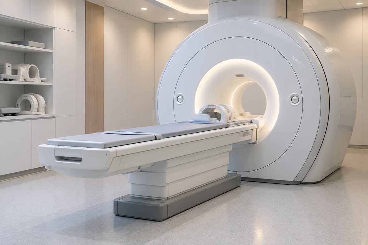
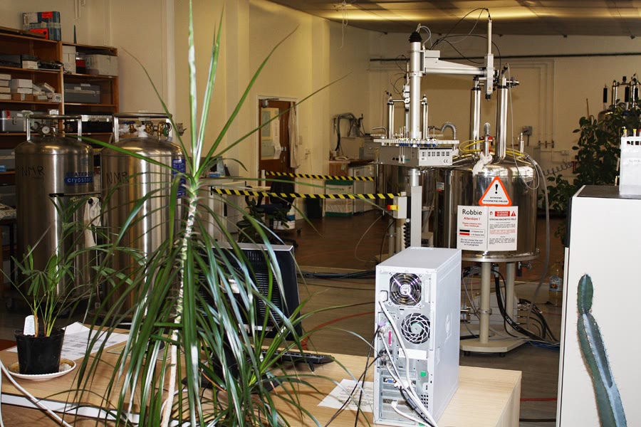
A hospital MRI scanner and the NMR spectrometer of a chemistry department work on the same principle. Each places hydrogen nuclei in a strong magnetic field, tips their magnetisation with a short pulse of radio waves, and listens to the faint signal it induces as it precesses and relaxes. The scanner turns the signal into an image of soft tissue; the spectrometer into a list of chemical shifts and couplings, and, with several pulses in a row, into two-dimensional maps that show which atom is bonded to which. This chapter explains what the pulses do, why the signal fades, and how two-dimensional spectra are read — the method by which most new organic structures are now solved.

You already know

The Year 1 volume interpreted ${}^1$ H NMR spectra: chemical shift, shielding, equivalent protons, integration, spin–spin coupling, coupling constants and multiplets. The Year 2 volume added ${}^{13}$ C NMR with broadband decoupling and DEPT, whose pulse sequence it took as given; the pulses are explained here. Chapter 2 treated spin as an angular momentum. From physics: a magnetic moment in a field has energy $-\boldsymbol\mu\cdot\mathbf B$ , and populations of levels follow the Boltzmann factor $\eu^{-\Delta E/kT}$ , developed in Chapter 10.

Left: a hospital MRI scanner. Right: an NMR laboratory; each superconducting magnet stands in its cryostat, refilled with liquid helium and liquid nitrogen from the dewars on the left. Photograph Shandchem, CC BY 2.0.

8.1 Nuclear spins in a magnetic field

Definition 8.1 (Nuclear spin quantum number, gyromagnetic ratio)

A nucleus has a spin angular momentum of quantum number $I$ , its nuclear spin quantum number ( $I = 0$ for $\ce{^{12}C}$ , $\ce{^{16}O}$ ; $\frac12$ for $\ce{^1H}$ , $\ce{^{13}C}$ , $\ce{^{15}N}$ , $\ce{^{19}F}$ , $\ce{^{31}P}$ ; 1 for $\ce{^2H}$ , $\ce{^{14}N}$ ), and a magnetic moment $\boldsymbol\mu = \gamma\hat{\mathbf I}$ proportional to it; $\gamma$ is the gyromagnetic ratio. Along a field $B_0$ (axis $z$ ), $\hat I_z$ takes the values $m_I\hbar$ , $m_I = -I, \dots, I$ .

Proposition 8.2 (Zeeman levels)

In a field $B_0$ the levels are $E_m = -m_I\gamma\hbar B_0$ ; the transitions $\Delta m_I = \pm1$ absorb at the frequency

\nu_0 = \frac{\gamma B_0}{2\pi}.

Proof. $E = -\boldsymbol\mu\cdot\mathbf B = -\gamma B_0\hat I_z$ , of eigenvalues $-\gamma B_0m_I\hbar$ . Adjacent levels differ by $\gamma\hbar B_0 = h\nu_0$ . ∎

Definition 8.3 (Larmor frequency)

$\nu_0 = \gamma B_0/2\pi$ is the Larmor frequency of the nucleus: the frequency of the resonance, and also the frequency at which its magnetic moment precesses about the field.

Example 8.4 (The common nuclei)

For a spin- $\frac12$ nucleus of moment $\mu$ , $\gamma/2\pi = \mu/(Ih) = 2\mu/h$ . With the measured moments: $\ce{^1H}$ $42.58\,\mathrm{MHz}/\mathrm{T}$ , $\ce{^{19}F}$ $40.08\,\mathrm{MHz}/\mathrm{T}$ , $\ce{^{31}P}$ $17.25\,\mathrm{MHz}/\mathrm{T}$ , $\ce{^{13}C}$ $10.71\,\mathrm{MHz}/\mathrm{T}$ , $\ce{^{15}N}$ $-4.32\,\mathrm{MHz}/\mathrm{T}$ . A “ $400\,\mathrm{MHz}$ spectrometer” has $B_0 = 9.4\,\mathrm{T}$ : its protons resonate at $400.2\,\mathrm{MHz}$ , its carbons at $100.7\,\mathrm{MHz}$ .

Proposition 8.5 (A tiny population difference)

For spin $\frac12$ at temperature $T$ , the excess of nuclei in the lower level is

\frac{N_\alpha - N_\beta}{N} \approx \frac{\gamma\hbar B_0}{2kT}.

Proof. $N_\beta/N_\alpha = \eu^{-\Delta E/kT} \approx 1 - \Delta E/kT$ since $\Delta E \ll kT$ ; so $(N_\alpha - N_\beta)/(N_\alpha + N_\beta) \approx \Delta E/2kT$ , with $\Delta E = \gamma\hbar B_0$ . ∎

For protons at $9.4\,\mathrm{T}$ and $300\,\mathrm{K}$ the excess is $3.2 \times 10^{-5}$ : only three nuclei in a hundred thousand contribute. Since both the excess and the voltage induced in the coil grow with $\gamma$ and $B_0$ , the signal grows roughly as $\gamma^3B_0^2$ : the reason for ever stronger magnets, and for the low sensitivity of nuclei with small $\gamma$ and low natural abundance such as $\ce{^{13}C}$ .

8.2 Pulses and the free induction decay

Definition 8.6 (Net magnetisation, rotating frame)

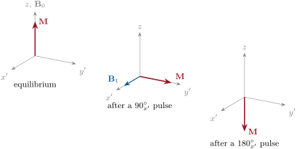
The net magnetisation $\mathbf M$ of a sample is the sum of its nuclear magnetic moments per unit volume; at equilibrium it is $M_0$ along $\mathbf B_0$ . The rotating frame is a set of axes $x'$ , $y'$ , $z$ turning about $z$ at the frequency of the radio waves applied; in it the precession at $\nu_0$ is seen slowed to the offset $\nu_0 - \nu_{\mathrm{rf}}$ .

Proposition 8.7 (Precession)

A magnetisation in a field obeys $\dd\mathbf M/\dd t = \gamma\,\mathbf M\times\mathbf B$ ; in a static field $B_0\mathbf e_z$ , its transverse component turns about $z$ at the angular frequency $\omega_0 = \gamma B_0$ while $M_z$ stays constant.

Partial proof. The equation is the classical torque equation for a magnetic moment carrying angular momentum, admitted from physics. With $\mathbf B = B_0\mathbf e_z$ : $\dot M_x = \gamma B_0M_y$ , $\dot M_y = -\gamma B_0M_x$ , $\dot M_z = 0$ , whose solution is $M_x + \iu M_y \propto \eu^{-\iu\gamma B_0t}$ : a rotation at $\omega_0$ (clockwise seen from $+z$ for $\gamma > 0$ ). ∎

Definition 8.8 (Radiofrequency pulse, flip angle)

A radiofrequency pulse is a short burst of radio waves at $\nu_{\mathrm{rf}} \approx \nu_0$ , whose magnetic field $B_1$ , fixed in the rotating frame along $x'$ , turns $\mathbf M$ about $x'$ . The angle turned is the flip angle $\theta = \gamma B_1t_p$ for a pulse of duration $t_p$ : a $90^\circ$ pulse brings $\mathbf M$ into the $x'y'$ plane, a $180^\circ$ pulse inverts it.

The magnetisation in the rotating frame. A 90 pulse about x' turns M from z to y' (with > 0 the rotation follows the left-hand rule about B_1, the usual convention); a 180 pulse inverts it. — The magnetisation in the rotating frame. A $90^\circ$ pulse about $x'$ turns $\mathbf M$ from $z$ to $y'$ (with $\gamma > 0$ the rotation follows the left-hand rule about $\mathbf B_1$ , the usual convention); a $180^\circ$ pulse inverts it.

Definition 8.9 (Free induction decay)

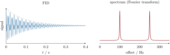
After a $90^\circ$ pulse, the transverse magnetisation precesses at the Larmor frequency and induces an oscillating voltage in the coil around the sample, which dies away as the magnetisation relaxes: the free induction decay (FID).

Theorem 8.10 (From the FID to the spectrum)

The Fourier transform of a decaying oscillation $\eu^{-t/T_2}\cos(2\pi\nu t)$ ( $t \ge 0$ ) is, near $\nu$ , a Lorentzian line of full width at half maximum $1/(\pi T_2)$ .

Proof. Write the signal $\eu^{-t/T_2}\eu^{2\pi\iu\nu t}$ and integrate: $\int_0^\infty\eu^{-t/T_2}\eu^{2\pi\iu(\nu - f)t}\dd t = \frac{1}{1/T_2 - 2\pi\iu(\nu - f)}$ , whose real part is $\frac{T_2}{1 + 4\pi^2T_2^2(f - \nu)^2}$ . It is maximal at $f = \nu$ and falls to half when $2\pi T_2|f - \nu| = 1$ , i.e. at $f - \nu = \pm1/(2\pi T_2)$ : a full width $1/(\pi T_2)$ . ∎

Left: the FID of two lines (offsets 100 and 250\, Hz, T_2 = 0.10\, s), beating as the two frequencies interfere inside an exponential envelope (dashed). Right: its Fourier transform, two Lorentzian lines 3.2\, Hz wide. — Left: the FID of two lines (offsets 100 and $250\,\mathrm{Hz}$ , $T_2 = 0.10\,\mathrm{s}$ ), beating as the two frequencies interfere inside an exponential envelope (dashed). Right: its Fourier transform, two Lorentzian lines $3.2\,\mathrm{Hz}$ wide.

Proposition 8.11 (Signal averaging)

Adding $N$ FIDs multiplies the signal by $N$ and the random noise by $\sqrt N$ : the signal-to-noise ratio grows as $\sqrt N$ .

Proof. The signal adds coherently. The noise of independent acquisitions has zero mean and variance $\sigma^2$ each; the variance of a sum of $N$ independent terms is $N\sigma^2$ (the propagation law of the Year 2 volume), so its standard deviation is $\sqrt N\sigma$ . ∎

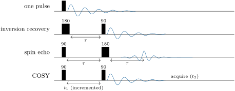
DEPT, which sorts ${}^{13}$ C signals by the number of attached hydrogens, applies a sequence of pulses to both protons and carbons separated by delays of $1/2J$ : the large proton magnetisation is transferred to the carbon through the one-bond coupling, which multiplies the carbon signal by about $\gamma_H/\gamma_C \approx 4$ , and the final proton pulse angle weights CH, $\ce{CH2}$ and $\ce{CH3}$ differently. The same idea — moving magnetisation between nuclei through their couplings — underlies the two-dimensional experiments below.

8.3 Relaxation

Definition 8.12 (Longitudinal and transverse relaxation times)

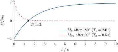
The return of $M_z$ to $M_0$ after a perturbation is exponential, with the longitudinal relaxation time $T_1$ (spin–lattice relaxation: energy given to the surroundings). The decay of the transverse magnetisation to zero is exponential with the transverse relaxation time $T_2 \le T_1$ (spin–spin relaxation: loss of phase coherence between spins).

Proposition 8.13 (Inversion recovery)

After a $180^\circ$ pulse, $M_z(t) = M_0(1 - 2\eu^{-t/T_1})$ ; it passes through zero at $t_{\mathrm{null}} = T_1\ln2$ .

Proof. The relaxation equation $\dd M_z/\dd t = (M_0 - M_z)/T_1$ with $M_z(0) = -M_0$ has the solution $M_0 - 2M_0\eu^{-t/T_1}$ , which vanishes when $\eu^{-t/T_1} = \frac12$ . ∎

Method 8.14 (Measuring $T_1$ and setting a quantitative recycle delay)

Run the sequence $180^\circ$ – $\tau$ – $90^\circ$ –acquire for a series of delays $\tau$ , waiting at least $5T_1$ between scans.
Fit each signal to $M_0(1 - 2\eu^{-\tau/T_1})$ , or read the null: $T_1 = t_{\mathrm{null}}/\ln2$ .
For quantitative integration with $90^\circ$ pulses, wait at least $5T_1$ of the slowest nucleus between scans: then $\eu^{-5} < 1\,\%$ of the magnetisation is missing.

Relaxation (model values). The inverted longitudinal magnetisation recovers through zero at T_1 2; the transverse magnetisation decays faster, with T_2. — Relaxation (model values). The inverted longitudinal magnetisation recovers through zero at $T_1\ln2$ ; the transverse magnetisation decays faster, with $T_2$ .

Definition 8.15 (Spin echo)

In the sequence $90^\circ$ – $\tau$ – $180^\circ$ – $\tau$ , spins that drifted apart in phase because of field inhomogeneities are refocused at time $2\tau$ , producing a spin echo; its amplitude decays with the true $T_2$ , free of the inhomogeneity of the magnet.

Definition 8.16 (Nuclear Overhauser effect)

Saturating or perturbing one spin changes, through their dipolar relaxation, the intensity of the signal of another spin close in space: the nuclear Overhauser effect (NOE). Its build-up rate is proportional to $r^{-6}$ , so it is seen only between nuclei less than about $0.5\,\mathrm{nm}$ apart, whether bonded or not.

8.4 Two-dimensional NMR

Definition 8.17 (Two-dimensional spectrum, cross peak, diagonal peak)

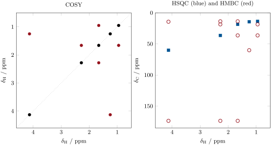
A two-dimensional spectrum is recorded by repeating a pulse sequence with an incremented delay $t_1$ before the acquisition time $t_2$ ; a double Fourier transform gives a map of intensity against two frequencies. A cross peak at $(\delta_1, \delta_2)$ shows that the nuclei at $\delta_1$ and $\delta_2$ are connected (by a coupling or by proximity); a diagonal peak at $(\delta, \delta)$ belongs to a single nucleus.

Definition 8.18 (COSY, HSQC, HMBC, NOESY)

COSY (correlation spectroscopy) correlates protons coupled to each other, usually through three bonds (H–C–C–H). HSQC (heteronuclear single-quantum coherence) correlates each carbon with the protons directly bonded to it. HMBC (heteronuclear multiple-bond correlation) correlates carbons with protons two or three bonds away, across quaternary carbons and heteroatoms. NOESY correlates protons close in space through the nuclear Overhauser effect.

Pulse sequences (time to the right; filled boxes: pulses, labelled with their flip angles in degrees; blue: the recorded signal). The spin echo peaks at 2 after the first pulse. — Pulse sequences (time to the right; filled boxes: pulses, labelled with their flip angles in degrees; blue: the recorded signal). The spin echo peaks at $2\tau$ after the first pulse.

Method 8.19 (Solving a structure with two-dimensional spectra)

From the formula, the ${}^1$ H integrals and the ${}^{13}$ C/DEPT spectrum, list the CH, $\ce{CH2}$ , $\ce{CH3}$ and quaternary carbons.
HSQC: attach each proton signal to its carbon.
COSY: join the protonated carbons into spin systems (chains of neighbours).
HMBC: join the spin systems across quaternary carbons, carbonyls and heteroatoms, where COSY is silent.
NOESY: fix relative configurations and conformations from through-space contacts.
Check every signal against the proposed structure.

Two-dimensional spectra of ethyl butanoate, CH3CH2CH2COOCH2CH3, drawn at its measured shifts. COSY: black, diagonal peaks; red, cross peaks between protons on neighbouring carbons — two spin systems, ethyl and propyl, with no cross peak across the ester oxygen. Right: HSQC peaks (squares) join each proton to its carbon; HMBC peaks (circles) show the OCH_2 protons (4.13\, ppm) and the CH_2C=O protons (2.28\, ppm) both reaching the carbonyl carbon at 173.6\, ppm. — Two-dimensional spectra of ethyl butanoate, $\ce{CH3CH2CH2COOCH2CH3}$ , drawn at its measured shifts. COSY: black, diagonal peaks; red, cross peaks between protons on neighbouring carbons — two spin systems, ethyl and propyl, with no cross peak across the ester oxygen. Right: HSQC peaks (squares) join each proton to its carbon; HMBC peaks (circles) show the OCH $_2$ protons ( $4.13\,\mathrm{ppm}$ ) and the CH $_2$ C=O protons ( $2.28\,\mathrm{ppm}$ ) both reaching the carbonyl carbon at $173.6\,\mathrm{ppm}$ .

8.5 Other nuclei and dynamics

Fluorine-19 and phosphorus-31, spin $\frac12$ , 100 % abundant and with large $\gamma$ , are almost as easy to observe as protons; their wide ranges of shifts make them precise probes of their environment (drugs, phosphates, ligands such as phosphines in Chapter 20). Nitrogen-15 is rare and weak, and is usually observed indirectly through the protons bonded to it. Coupling between different nuclei is removed by decoupling, as for ${}^{13}$ C in the Year 2 volume.

Definition 8.20 (Coalescence temperature)

When a nucleus exchanges between two environments of shifts separated by $\Delta\nu$ (in hertz), its two lines broaden as the exchange speeds up and merge into one at the coalescence temperature $T_c$ .

Proposition 8.21 (Rate at coalescence)

For two equally populated sites without coupling, the exchange rate constant at coalescence is $k_c = \pi\Delta\nu/\sqrt2$ .

Proof. Admitted at this level. ∎

The derivation, from the Bloch equations with exchange, is treated in more advanced courses. With the Eyring equation (Chapter 12) the rate gives the barrier: dynamic NMR measures rotations about amide bonds, ring flips and ligand exchanges with barriers of 40 to $100\,\mathrm{kJ}/\mathrm{mol}$ .

Example 8.22 (An MRI image)

In magnetic resonance imaging a field gradient makes the Larmor frequency of the water protons depend on position, so that the Fourier transform of the signal is a map of where they are. Contrast comes from relaxation: the repetition time and echo delays are chosen to weight the image by $T_1$ or by $T_2$ , which differ between tissues; contrast agents containing gadolinium shorten the $T_1$ of nearby water (Chapter 24).

In the lab — Preparing a spectrometer

The sample, dissolved in a deuterated solvent, is lowered into the probe. The spectrometer locks on the deuterium signal to compensate the slow drift of the field; the probe is tuned and matched to the frequency of each nucleus; the field is made homogeneous over the sample by adjusting the shim coils until the lines are narrow. The magnet’s field is permanent: steel tools, credit cards and pacemakers are kept outside the marked safety line.

History — From resonance to two dimensions

Felix Bloch and Edward Purcell detected nuclear magnetic resonance in bulk matter in 1946 (Nobel Prize in Physics, 1952). Richard Ernst introduced pulsed Fourier-transform NMR in 1966 and, following an idea of Jean Jeener, two-dimensional spectroscopy in the 1970s (Nobel Prize in Chemistry, 1991).

8.6 Exercises

Exercise 8.1 ★

Compute the Larmor frequencies of $\ce{^1H}$ , $\ce{^{13}C}$ and $\ce{^{19}F}$ at $14.1\,\mathrm{T}$ ( $\gamma/2\pi = 42.58$ , 10.71 and $40.08\,\mathrm{MHz}/\mathrm{T}$ ).

Solution

Solution of Exercise 8.1.

$\nu_0 = (\gamma/2\pi)B_0$ : $\ce{^1H}$ $600.4\,\mathrm{MHz}$ , $\ce{^{13}C}$ $151.0\,\mathrm{MHz}$ , $\ce{^{19}F}$ $565.1\,\mathrm{MHz}$ .

Exercise 8.2 ★

Compute the relative excess of protons in the lower level at $9.4\,\mathrm{T}$ and $300\,\mathrm{K}$ . By how much does it change at $4\,\mathrm{K}$ ?

Solution

Solution of Exercise 8.2.

$h\nu_0/2kT = 6.626\times10^{-34} \times 400.2\times10^6/(2 \times 1.381\times10^{-23} \times 300) = 3.2 \times 10^{-5}$ . At $4\,\mathrm{K}$ it is 75 times larger, $2.4 \times 10^{-3}$ (the approximation still holds).

Exercise 8.3 ★

A $90^\circ$ pulse lasts $10\,\text{µ}\mathrm{s}$ for protons. What is $\gamma B_1/2\pi$ ? How long is a $180^\circ$ pulse, and what does a $5\,\text{µ}\mathrm{s}$ pulse do?

Solution

Solution of Exercise 8.3.

$\theta = \gamma B_1t_p = \pi/2$ in $10\,\text{µ}\mathrm{s}$ : $\gamma B_1/2\pi = 1/(4 \times 10\,\text{µ}\mathrm{s}) = 25\,\mathrm{kHz}$ . A $180^\circ$ pulse lasts $20\,\text{µ}\mathrm{s}$ ; $5\,\text{µ}\mathrm{s}$ gives $45^\circ$ .

Exercise 8.4 ★

A line is $3.2\,\mathrm{Hz}$ wide at half height. What is $T_2$ (assuming a perfectly homogeneous field)?

Solution

Solution of Exercise 8.4.

$T_2 = 1/(\pi \times 3.2) = 0.10\,\mathrm{s}$ .

Exercise 8.5 ★★

Using signal $\propto\gamma^3$ per nucleus and the 1.1 % natural abundance of $\ce{^{13}C}$ , compare the sensitivity of ${}^{13}$ C and ${}^1$ H NMR. How many more scans does a ${}^{13}$ C spectrum need for the same signal-to-noise ratio?

Solution

Solution of Exercise 8.5.

$(10.71/42.58)^3 = 0.0159$ , times 0.011: $1.75 \times 10^{-4}$ , about 1/5700 of the proton signal. Since S/N $\propto\sqrt N$ , equal S/N needs $5700^2 \approx 3 \times 10^{7}$ times more scans — impossible, which is why ${}^{13}$ C spectra use more concentrated samples, decoupling and polarisation transfer.

Exercise 8.6 ★★

In an inversion-recovery experiment the signal of a carbon vanishes at $\tau = 1.39\,\mathrm{s}$ . Find $T_1$ and the recycle delay for quantitative work.

Solution

Solution of Exercise 8.6.

$T_1 = 1.39/\ln2 = 2.0\,\mathrm{s}$ ; recycle delay $\ge 5T_1 = 10\,\mathrm{s}$ .

Exercise 8.7 ★★

In the COSY spectrum of butanone, $\ce{CH3COCH2CH3}$ , which cross peaks appear? Which carbons show HMBC peaks from the singlet methyl protons?

Solution

Solution of Exercise 8.7.

COSY: one cross peak, between the $\ce{CH2}$ quartet and the $\ce{CH3}$ triplet of the ethyl group; the $\ce{CH3CO}$ singlet couples to nothing. HMBC from the singlet methyl: the carbonyl carbon (two bonds) and the $\ce{CH2}$ carbon (three bonds).

Exercise 8.8 ★★

Two methyl signals of an amide, $50\,\mathrm{Hz}$ apart at low temperature, coalesce at $330\,\mathrm{K}$ . Compute the exchange rate at coalescence and the Gibbs energy of activation with $\Delta G^\ddagger = RT_c\ln(k_BT_c/hk_c)$ .

Solution

Solution of Exercise 8.8.

$k_c = \pi \times 50/\sqrt2 = 111\,\mathrm{s}^{-1}$ . $\Delta G^\ddagger = 8.314 \times 330 \times \ln(6.88\times10^{12}/111) = 68\,\mathrm{kJ}/\mathrm{mol}$ .

Exercise 8.9 ★★

An NOE between protons H $_a$ and H $_b$ is four times stronger than between H $_a$ and H $_c$ , at $0.30\,\mathrm{nm}$ . Estimate the H $_a$ –H $_b$ distance.

Solution

Solution of Exercise 8.9.

NOE $\propto r^{-6}$ : $r_b = 0.30 \times 4^{-1/6} = 0.24\,\mathrm{nm}$ .

Exercise 8.10 ★★★

Show, by solving $\dd\mathbf M/\dd t = \gamma\mathbf M\times\mathbf B_1$ in the rotating frame with $\mathbf B_1$ along $x'$ , that a pulse rotates $\mathbf M$ by $\gamma B_1t_p$ about $x'$ .

Solution

Solution of Exercise 8.10.

In the rotating frame on resonance only $\mathbf B_1 = B_1\mathbf e_{x'}$ remains: $\dot M_{x'} = 0$ , $\dot M_{y'} = \gamma B_1M_z$ , $\dot M_z = -\gamma B_1M_{y'}$ (components of $\gamma\mathbf M\times\mathbf B_1$ ). So $M_{x'}$ is constant and $(M_{y'}, M_z)$ turns at the angular rate $\gamma B_1$ : after $t_p$ , by the angle $\gamma B_1t_p$ about $x'$ .

Exercise 8.11 ★★★

Explain why the spin echo refocuses the dephasing due to an inhomogeneous field but not that due to random interactions between spins. Which time constant does the echo amplitude measure?

Solution

Solution of Exercise 8.11.

A spin in a slightly stronger field gains phase at a constant extra rate during $\tau$ ; the $180^\circ$ pulse reverses its phase, and it loses exactly the same amount during the second $\tau$ : all such spins realign at $2\tau$ . Random spin–spin interactions fluctuate in time and do not repeat in the second interval: their dephasing is not undone. The echo amplitude decays with the true $T_2$ .

Exercise 8.12 ★★★

Propose the structure of a compound $\ce{C4H8O2}$ whose ${}^1$ H spectrum shows a quartet (2H, 4.12 ppm), a singlet (3H, 2.05 ppm) and a triplet (3H, 1.26 ppm), and whose HMBC spectrum correlates the quartet protons with a carbon at 171 ppm (data of the exercise). Which other ester of the same formula would give a different HMBC pattern, and how?

Solution

Solution of Exercise 8.12.

Ethyl ethanoate, $\ce{CH3COOCH2CH3}$ : $\ce{OCH2}$ quartet (4.12), $\ce{CH3CO}$ singlet (2.05), $\ce{CH3}$ triplet; the quartet protons see the carbonyl carbon three bonds away, through the ester oxygen. Methyl propanoate, $\ce{CH3CH2COOCH3}$ , would show its quartet near 2.3 ppm (on a carbon near 27 ppm in HSQC, not 60) and a singlet $\ce{OCH3}$ near 3.7 ppm whose HMBC peak to the carbonyl crosses the oxygen.

8.7 Problem: The Pineapple Ester in Two Dimensions

Problem 8.1

Weekend problem — ethyl butanoate solved again, from two-dimensional spectra: spin systems from COSY, carbons from HSQC, the ester linkage from HMBC, and the delay needed for a quantitative carbon spectrum

An ester $\ce{C6H12O2}$ from the aroma of pineapple shows ${}^1$ H signals at 4.13 (2H, q), 2.28 (2H, t), 1.66 (2H, m), 1.25 (3H, t) and 0.95 ppm (3H, t), and ${}^{13}$ C signals at 173.6, 60.1, 36.3, 18.6, 14.3 and 13.7 ppm, recorded at $9.4\,\mathrm{T}$ . Its 2D spectra are those of the figure of section 4. Data of the problem: the $T_1$ values of the carbons are about $20\,\mathrm{s}$ for the carbonyl and 2 to $6\,\mathrm{s}$ for the others.

Part I — One dimension.

Compute the degree of unsaturation of $\ce{C6H12O2}$ .
Which ${}^{13}$ C signal is the carbonyl? Which is the carbon bonded to oxygen?
How many protonated carbons are there? What would DEPT-135 show?
At $9.4\,\mathrm{T}$ , what are the Larmor frequencies of ${}^1$ H and ${}^{13}$ C?
The coupling of the quartet is $7.2\,\mathrm{Hz}$ . How wide, in ppm, is the quartet at $400\,\mathrm{MHz}$ ?
Why can the 1D spectra alone leave the order of the fragments open?

Part II — COSY.

List the cross peaks of the COSY map.
Deduce the two spin systems.
Why is there no cross peak between 4.13 and 2.28 ppm?
Which proton signal is coupled to two others? Explain its multiplicity.
What would a cross peak between 0.95 and 1.25 ppm have meant?
Draw the two fragments.

Part III — HSQC and HMBC.

From the HSQC, assign each carbon to its protons.
Which two methyl carbons are distinguished only by the HSQC?
Which HMBC peak links the ethyl fragment to the carbonyl, and through how many bonds?
Which HMBC peaks link the propyl fragment to the carbonyl?
Deduce the structure, and exclude its isomer propyl propanoate.
Why are HMBC peaks across four bonds or more usually absent?

Part IV — A quantitative carbon spectrum.

Why are the integrals of an ordinary ${}^{13}$ C spectrum not proportional to the number of carbons?
What fraction of its equilibrium magnetisation does the carbonyl recover if scans are repeated every $5\,\mathrm{s}$ with $90^\circ$ pulses (starting each time from zero)?
What fraction after $5T_1$ ?
Besides relaxation, which effect of proton decoupling distorts carbon integrals, and how is it suppressed?
With a delay of $5T_1$ , how long do 256 scans take?
State the result: the minimum recycle delay for a quantitative ${}^{13}$ C spectrum of this ester.

Solution

Solution of Problem 8.1.

1. $(2 \times 6 + 2 - 12)/2 = 1$ : one C=O. 2. 173.6 ppm: the ester carbonyl; 60.1 ppm: the $\ce{OCH2}$ . 3. Five; DEPT-135: $\ce{CH2}$ negative (60.1, 36.3, 18.6), $\ce{CH3}$ positive (14.3, 13.7), the carbonyl absent. 4. $400.2\,\mathrm{MHz}$ and $100.7\,\mathrm{MHz}$ . 5. $3J = 21.6\,\mathrm{Hz} = 0.054\,\mathrm{ppm}$ . 6. The multiplicities show which groups are neighbours inside each fragment, but not how the fragments join across the oxygen and the carbonyl. 7. 4.13–1.25; 2.28–1.66; 1.66–0.95 (and the symmetric ones). 8. $\ce{OCH2CH3}$ (4.13, 1.25) and $\ce{CH2CH2CH3}$ (2.28, 1.66, 0.95). 9. The $\ce{OCH2}$ and $\ce{CH2C=O}$ protons are separated by the oxygen and the carbonyl carbon: five bonds, no resolved coupling. 10. 1.66 ppm, between $\ce{CH2}$ and $\ce{CH3}$ : coupled to 2 + 3 = 5 protons with similar $J$ , a sextet (a multiplet). 11. Coupled methyls, hence two $\ce{CH3}$ on adjacent carbons (a $\ce{CH3-CH3}$ unit): impossible here. 12. $\ce{-O-CH2-CH3}$ and $\ce{-CH2-CH2-CH3}$ , plus the $\ce{C=O}$ . 13. 4.13/60.1; 2.28/36.3; 1.66/18.6; 1.25/14.3; 0.95/13.7. 14. 14.3 (ethyl $\ce{CH3}$ ) and 13.7 ppm (butanoyl $\ce{CH3}$ ), only $0.6\,\mathrm{ppm}$ apart. 15. 4.13 ppm to 173.6 ppm: H–C–O–C, three bonds. 16. 2.28 ppm (two bonds) and 1.66 ppm (three bonds) to 173.6 ppm. 17. $\ce{CH3CH2CH2C(=O)OCH2CH3}$ , ethyl butanoate. Propyl propanoate would put an $\ce{OCH2}$ triplet (not a quartet) near 4.0 ppm and a quartet near 2.3 ppm. 18. Four-bond couplings are usually below 1 Hz; the HMBC delay, tuned to 5–10 Hz, does not select them. 19. Carbons relax at different rates and receive different nuclear Overhauser enhancements from decoupling. 20. $1 - \eu^{-5/20} = 0.22$ : the carbonyl is under-represented by a factor 4. 21. $1 - \eu^{-5} = 0.993$ . 22. The NOE from proton decoupling, different for each carbon; it is removed by inverse-gated decoupling (decoupler on only during acquisition). 23. $256 \times 100\,\mathrm{s} = 25\,600\,\mathrm{s}$ , about 7 hours. 24. $5T_1$ of the carbonyl carbon: $100\,\mathrm{s}$ between scans.

Terms defined in this chapter

See all 852 terms in the glossary