University Chemistry — Year 3 · Bachelor Year 3

7Electronic Spectroscopy and Photophysics

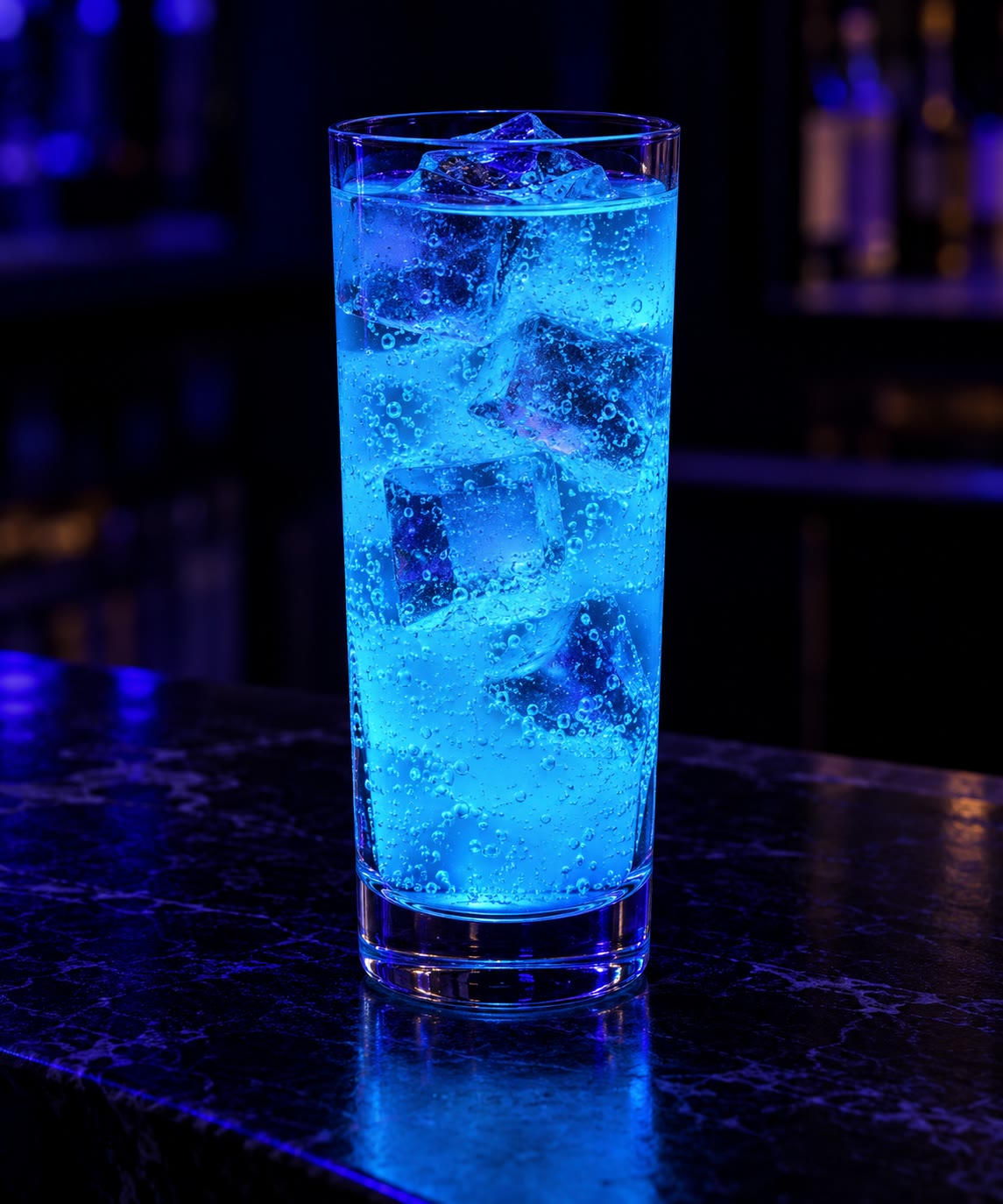
Under the ultraviolet lamp of a dark bar, a glass of tonic water glows a pale, ghostly blue. The quinine it contains absorbs ultraviolet light, which the eye cannot see, and gives part of it back a few nanoseconds later as visible blue light. Absorption, a short life in an excited state, emission at a longer wavelength, the energy that does not come back as light: the fate of an excited molecule is a competition between processes with rate constants, and its spectrum is shaped by the vibrations of the molecule and by the symmetry rules of Chapter 5. This chapter studies electronic transitions and what happens after them, the subject called photophysics; Chapter 14 adds the cases in which the excited molecule reacts.

You already know

The Year 1 volume measured absorbance with the Beer–Lambert law, $A = \varepsilon\ell c$ , defined the molar absorption coefficient, chromophores and conjugated systems, and related colour to the absorption maximum. The Year 2 volume named the frontier orbitals HOMO and LUMO. Chapter 2 defined singlet and triplet states; Chapter 5 the vanishing-integral theorem; Chapter 6 the vibrational levels of a bond.

Left: tonic water glowing blue under an ultraviolet lamp. Right: fluorite in daylight and fluorescing under ultraviolet light; the mineral gave fluorescence its name. Photograph Masha Milshina, CC BY 4.0.

7.1 Electronic transitions and their selection rules

Definition 7.1 (Transition dipole moment, oscillator strength)

The transition dipole moment between states $\Psi_i$ and $\Psi_f$ is $\boldsymbol\mu_{fi} = \langle\Psi_f|\hat{\boldsymbol\mu}|\Psi_i \rangle$ , with $\hat{\boldsymbol\mu} = -e\sum_k\mathbf r_k$ (plus the nuclear charges, which cancel between orthogonal states). The oscillator strength $f$ is the dimensionless measure of the intensity of a band, about 1 for the strongest transitions.

Proposition 7.2 (Intensity and oscillator strength)

The integrated absorption of a band is proportional to $|\boldsymbol\mu_{fi}|^2$ , and in practice

f \approx 4.32\times10^{-9}\int\varepsilon(\tilde\nu)\,\dd\tilde\nu,

with $\varepsilon$ in $\mathrm{L}\,\mathrm{mol}^{-1}\,\mathrm{cm}^{-1}$ and $\tilde\nu$ in $\mathrm{cm}^{-1}$ .

Proof. Admitted at this level. ∎

The proportionality comes from time-dependent perturbation theory and the numerical factor from the classical oscillator; both are treated in more advanced courses. What matters here is that $f$ is large only when $\boldsymbol\mu_{fi}$ is, and that symmetry can force it to zero.

Theorem 7.3 (The spin selection rule)

An electric-dipole transition between states of different total spin is forbidden: $\Delta S = 0$ .

Proof. Each state is a product of a spatial and a spin function, $\Psi = \phi\,\chi$ . The dipole operator acts on positions only, so $\langle\phi_f\chi_f|\hat{\boldsymbol\mu}| \phi_i\chi_i\rangle = \langle\phi_f|\hat{\boldsymbol\mu}|\phi_i\rangle\langle\chi_f|\chi_i\rangle$ . Spin functions of different $S$ are eigenfunctions of $\hat S^2$ with different eigenvalues, hence orthogonal (Theorem 1.4): the second factor vanishes. ∎

Theorem 7.4 (The Laporte rule)

In a molecule with a centre of inversion, an electric-dipole transition must change parity: $g \leftrightarrow u$ is allowed, $g \leftrightarrow g$ and $u \leftrightarrow u$ are forbidden. This is the Laporte rule.

Proof. The components of $\hat{\boldsymbol\mu}$ change sign under inversion: they are $u$ . The product $\Gamma_f\otimes\Gamma_\mu\otimes\Gamma_i$ is $g$ only if $\Gamma_f$ and $\Gamma_i$ have opposite parities; otherwise it is $u$ and cannot contain the totally symmetric representation (Theorem 5.18). ∎

The two rules are strict for the idealised states; real molecules relax them — spin–orbit coupling mixes singlet and triplet character, vibrations remove the centre of symmetry for an instant — and the “forbidden” transitions appear, weakly. The $d$ – $d$ bands of octahedral complexes, Laporte forbidden and weak, owe their colour to this relaxation (Chapter 18).

Definition 7.5 (Charge-transfer transition)

A charge-transfer transition moves an electron from an orbital located mainly on one part of a system (a donor) to an orbital located mainly on another (an acceptor); its transition dipole is large, its band intense and broad, and its energy sensitive to the polarity of the solvent.

Method 7.6 (Assigning an absorption band)

$\varepsilon_{\max}$ above about $10^{4}\,\mathrm{L}\,\mathrm{mol}^{-1}\,\mathrm{cm}^{-1}$ : an allowed transition ( $\pi\to\pi^*$ of a conjugated system, or charge transfer).
$\varepsilon_{\max}$ of 10 to a few hundred: a forbidden one ( $n\to\pi^*$ , symmetry-forbidden; $d$ – $d$ , Laporte-forbidden).
$\varepsilon_{\max}$ below 1: spin-forbidden.
An $n\to\pi^*$ band moves to shorter wavelengths in protic solvents (the lone pair is stabilised by hydrogen bonds), a $\pi\to\pi^*$ band usually to longer ones.

7.2 The Franck–Condon principle

Theorem 7.7 (Franck–Condon principle)

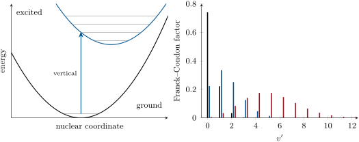
Within the Born–Oppenheimer approximation, and if the transition dipole depends little on the nuclear positions, the intensity of the vibronic transition from vibrational level $v''$ of the lower electronic state to level $v'$ of the upper one is proportional to $|\langle\chi_{v'}|\chi_{v''}\rangle|^2$ , the square of the overlap of the two vibrational wavefunctions: this is the Franck–Condon principle. Electronic transitions are vertical: the nuclei do not move while the electrons jump.

Proof. With $\Psi = \psi_{\mathrm{el}}(\mathbf r;R)\chi_v(R)$ , the transition moment is $\int\chi_{v'}^*\big[\int\psi'^*_{\mathrm{el}}\hat\mu\psi''_{\mathrm{el}}\dd\mathbf r\big] \chi_{v''}\,\dd R$ . The bracket is the electronic transition moment $\mu_{\mathrm{el}}(R)$ ; taken as constant (the Condon approximation), it comes out of the integral, leaving $\mu_{\mathrm{el}}\langle\chi_{v'}|\chi_{v''}\rangle$ . ∎

Definition 7.8 (Vibronic transition, progression, Franck–Condon factor)

A vibronic transition changes the electronic and vibrational states together; the lines $v' \leftarrow 0$ for $v' = 0, 1, 2, \dots$ form a vibronic progression; the Franck–Condon factor of a vibronic line is $|\langle\chi_{v'}|\chi_{v''}\rangle|^2$ .

Proposition 7.9 (Displaced oscillators)

If both states are harmonic with the same frequency and the upper minimum is displaced by $\Delta$ (in units of $\sqrt{\hbar/m\omega}$ ), the Franck–Condon factors from $v'' = 0$ form a Poisson distribution, $|\langle v'|0\rangle|^2 = \eu^{-S}S^{v'}/v'!$ , with $S = \Delta^2/2$ ; the strongest line is near $v' = S$ .

Proof. Admitted at this level. ∎

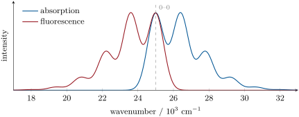
The general proof uses the ladder operators of Chapter 1; this chapter’s figure data checks the formula against direct integration. A small displacement gives one strong 0–0 line; a large one a long progression whose strongest member is far from the 0–0 line.

Left: a vertical transition from the lowest level of the ground state lands where the excited curve, displaced to longer bond length, is high above its minimum (drawn for S = 1.5). Right: Franck–Condon factors of the progression for S = 0.3 (black), 1.5 (blue) and 5 (red); each set adds up to 1. — Left: a vertical transition from the lowest level of the ground state lands where the excited curve, displaced to longer bond length, is high above its minimum (drawn for $S = 1.5$ ). Right: Franck–Condon factors of the progression for $S = 0.3$ (black), 1.5 (blue) and 5 (red); each set adds up to 1.

Example 7.10 (Iodine)

Iodine vapour is violet because its B $\leftarrow$ X band absorbs yellow-green light. The bond lengthens from $266.6\,\mathrm{pm}$ in the ground state to $302.5\,\mathrm{pm}$ in the B state. In the displaced-oscillator model with the B-state frequency ( $125.7\,\mathrm{cm}^{-1}$ ), $\Delta R = 35.8\,\mathrm{pm}$ gives $S \approx 15$ : the absorption is a long progression whose strongest lines end on high vibrational levels of the B state, and whose continuation runs into the dissociation continuum.

7.3 The fates of an excited state: the Jablonski diagram

Definition 7.11 (Jablonski diagram)

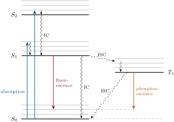
A Jablonski diagram shows the electronic states of a molecule (singlets $S_0, S_1, S_2, \dots$ in one column, triplets $T_1, T_2, \dots$ in another), their vibrational levels, and the processes connecting them: radiative ones as straight arrows, radiationless ones as wavy arrows.

Definition 7.12 (Radiationless processes)

Vibrational relaxation brings an excited molecule to the lowest vibrational level of its electronic state by collisions, in picoseconds. Internal conversion is a radiationless transition between states of the same multiplicity ( $S_2 \to S_1$ , $S_1 \to S_0$ ); intersystem crossing one between states of different multiplicity ( $S_1 \to T_1$ , $T_1 \to S_0$ ).

Definition 7.13 (Luminescence, fluorescence, phosphorescence, Stokes shift)

Luminescence is emission of light by an excited molecule. Fluorescence is spin-allowed emission, usually $S_1 \to S_0$ , fast (nanoseconds); phosphorescence is spin-forbidden emission, usually $T_1 \to S_0$ , slow (milliseconds to seconds). The Stokes shift is the difference between the absorption and emission maxima, in energy.

A Jablonski diagram. Straight arrows: absorption (blue), fluorescence (red), phosphorescence (orange); wavy arrows: vibrational relaxation and internal conversion (IC); dashed wavy arrows: intersystem crossing (ISC). Emission starts from the lowest vibrational level of S_1 or T_1 and may end on any level of S_0. — A Jablonski diagram. Straight arrows: absorption (blue), fluorescence (red), phosphorescence (orange); wavy arrows: vibrational relaxation and internal conversion (IC); dashed wavy arrows: intersystem crossing (ISC). Emission starts from the lowest vibrational level of $S_1$ or $T_1$ and may end on any level of $S_0$ .

Proposition 7.14 (Kasha’s rule)

Luminescence occurs, with very few exceptions, from the lowest excited state of a given multiplicity ( $S_1$ or $T_1$ ), whatever state was first excited: Kasha’s rule.

Status. Established experimentally; the reason is that internal conversion between upper excited states, which lie close together, is far faster than emission, while the gap $S_1$ – $S_0$ is large. ∎

Proposition 7.15 (Mirror image)

If the excited and ground states have similar vibrational structure, the fluorescence band is the mirror image of the first absorption band about their common 0–0 line; the emission lies at longer wavelengths (Stokes shift).

Proof. Absorption goes from $v'' = 0$ to the levels $v'$ of $S_1$ , at $E_{00} + v'h\nu'$ ; emission from $v' = 0$ to the levels $v''$ of $S_0$ , at $E_{00} - v''h\nu''$ . With equal frequencies and the same Franck–Condon factors (equal displacement), the two progressions are symmetric about $E_{00}$ . ∎

Absorption and fluorescence of a model molecule (S = 1, vibrational quantum 1400\, cm-1): mirror images about the 0–0 line; the maxima are separated by the Stokes shift. — Absorption and fluorescence of a model molecule ( $S = 1$ , vibrational quantum $1400\,\mathrm{cm}^{-1}$ ): mirror images about the 0–0 line; the maxima are separated by the Stokes shift.

7.4 Kinetics of excited states

After excitation, the population of $S_1$ decays by every process open to it, each first order: radiative decay $k_r$ , internal conversion $k_{\mathrm{IC}}$ , intersystem crossing $k_{\mathrm{ISC}}$ .

Definition 7.16 (Excited-state lifetime, radiative lifetime)

The excited-state lifetime is $\tau = 1/\sum k$ , the time constant of the exponential decay of the excited population. The radiative lifetime $\tau_r = 1/k_r$ is the lifetime the state would have if emission were its only fate.

Definition 7.17 (Quantum yield)

The quantum yield of a process that follows the absorption of light is the number of events of that process divided by the number of photons absorbed. The fluorescence quantum yield $\Phi_F$ is the number of photons emitted as fluorescence per photon absorbed.

Proposition 7.18 (Quantum yield and lifetime)

$\Phi_F = k_r/(k_r + k_{\mathrm{IC}} + k_{\mathrm{ISC}}) = k_r\tau = \tau/\tau_r$ ; likewise $\Phi_{\mathrm{ISC}} = k_{\mathrm{ISC}}\tau$ , and the yields of the competing processes add up to 1.

Proof. $\dd[S_1]/\dd t = -(k_r + k_{\mathrm{IC}} + k_{\mathrm{ISC}})[S_1]$ , so $[S_1] = [S_1]_0\eu^{-t/\tau}$ . The number of photons emitted is $\int_0^\infty k_r[S_1]\,\dd t = k_r\tau[S_1]_0$ , out of $[S_1]_0$ excited molecules. The same integral with each $k$ gives each yield, and their sum is $\tau\sum k = 1$ . ∎

Definition 7.19 (Fluorescence quencher, dynamic and static quenching)

A fluorescence quencher is a species that reduces fluorescence. In dynamic quenching it deactivates the excited molecule on collision, adding a rate $k_q[Q]$ and shortening the lifetime; in static quenching it forms a non-fluorescent complex with the ground-state molecule, reducing the intensity without changing the lifetime of the molecules that still emit.

Theorem 7.20 (Stern–Volmer equation)

For dynamic quenching,

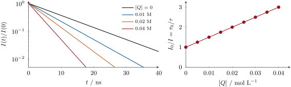
\frac{I_0}{I} = \frac{\tau_0}{\tau} = 1 + k_q\tau_0[Q] = 1 + K_{SV}[Q],

the Stern–Volmer equation, where $I_0$ , $\tau_0$ are measured without quencher and $K_{SV} = k_q\tau_0$ .

Proof. With quencher, $\tau = 1/(k_0 + k_q[Q])$ with $k_0 = 1/\tau_0$ , so $\tau_0/\tau = 1 + k_q\tau_0[Q]$ . The intensity is proportional to $\Phi_F = k_r\tau$ , so $I_0/I = \tau_0/\tau$ . ∎

Dynamic quenching of a model fluorophore (_0 = 10\, ns, k_q = 5 × 109\, L\, mol-1\, s-1). Left: fluorescence decays, straight lines on a log scale, steeper with more quencher. Right: the Stern–Volmer line, of slope K_SV = k_q _0 = 50\, L/ mol. — Dynamic quenching of a model fluorophore ( $\tau_0 = 10\,\mathrm{ns}$ , $k_q = 5 \times 10^{9}\,\mathrm{L}\,\mathrm{mol}^{-1}\,\mathrm{s}^{-1}$ ). Left: fluorescence decays, straight lines on a log scale, steeper with more quencher. Right: the Stern–Volmer line, of slope $K_{SV} = k_q\tau_0 = 50\,\mathrm{L}/\mathrm{mol}$ .

Method 7.21 (Relative fluorescence quantum yield)

Choose a standard of known $\Phi_{\mathrm{std}}$ absorbing at the same excitation wavelength.
Prepare dilute solutions ( $A < 0.1$ , to avoid re-absorption) and record their absorbances $A$ and integrated emission spectra $F$ under identical conditions.
$\Phi = \Phi_{\mathrm{std}}\,\dfrac{F}{F_{\mathrm{std}}}\,\dfrac{A_{\mathrm{std}}}{A}\, \dfrac{n^2}{n_{\mathrm{std}}^2}$ , the last factor correcting for the refractive indices of the solvents.

Method 7.22 (Analysing quenching data)

Plot $I_0/I$ against $[Q]$ ; a straight line through 1 gives $K_{SV}$ .
Measure lifetimes too: if $\tau_0/\tau$ follows the same line, the quenching is dynamic, and $k_q = K_{SV}/\tau_0$ ; if $\tau$ does not change, it is static.
Compare $k_q$ with the diffusion limit, about $10^{10}\,\mathrm{L}\,\mathrm{mol}^{-1}\,\mathrm{s}^{-1}$ in water (Chapter 12): a $k_q$ close to it means nearly every encounter quenches.

Example 7.23 (Quinine and anthracene)

Quinine sulfate in $0.5\,\mathrm{M}$ sulfuric acid absorbs at $349\,\mathrm{nm}$ with $\varepsilon = 5700\,\mathrm{L}\,\mathrm{mol}^{-1}\,\mathrm{cm}^{-1}$ and fluoresces with $\Phi_F = 0.546$ , which makes it the classic standard for relative quantum yields. Anthracene in cyclohexane absorbs at $356\,\mathrm{nm}$ and has $\Phi_F = 0.36$ ; most of the rest of its excited molecules cross to the triplet.

7.5 Applications

Fluorescence is detected against a dark background, which makes fluorimetry a hundred to a thousand times more sensitive than absorption spectroscopy: nanomolar concentrations of a fluorescent compound are measured routinely. Fluorescent probes report on their surroundings through their wavelength, yield or lifetime (polarity, pH, the binding of an ion); energy transfer between two fluorophores, efficient only over a few nanometres, measures distances in proteins. Phosphorescent complexes of heavy metals, in which spin–orbit coupling makes intersystem crossing efficient, harvest triplets in the light-emitting diodes of display screens.

In the lab — Time-correlated single-photon counting

To measure a nanosecond lifetime, the sample is excited by a pulsed laser diode at a megahertz repetition rate, and for each pulse the delay of the first fluorescence photon detected is recorded. After millions of pulses the histogram of delays is the decay curve, from which $\tau$ is fitted, with the instrument response measured on a scattering solution. The ultraviolet source is enclosed; the operator works with goggles that block its wavelength.

History — Stokes, 1852

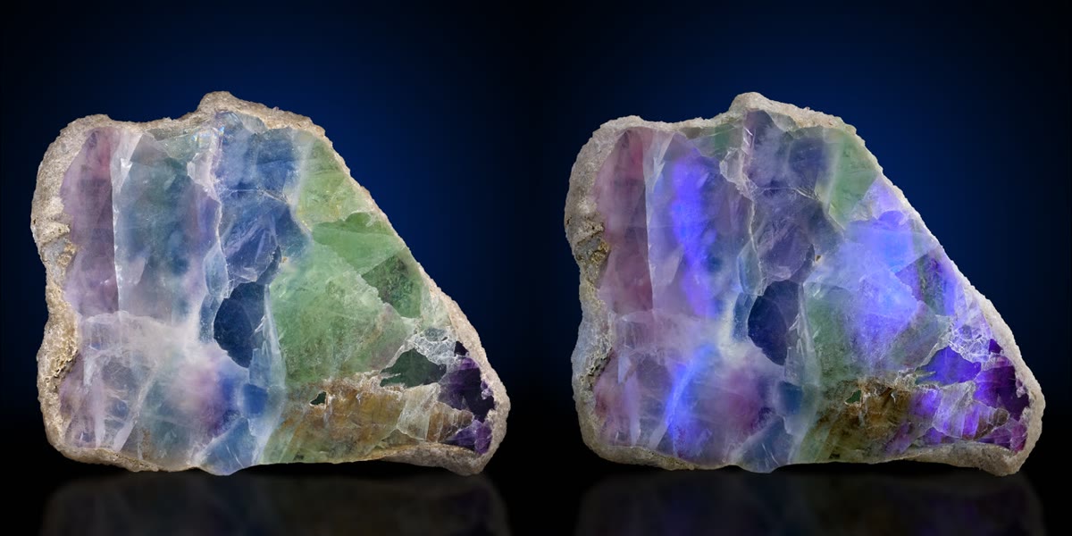
George Gabriel Stokes passed sunlight through a violet glass and a prism into a solution of quinine, and saw blue light emerge from the region lit by invisible ultraviolet rays: the emitted light always had a longer wavelength than the light absorbed. He called the phenomenon fluorescence, after the mineral fluorite, which glows the same way.

7.6 Exercises

Exercise 7.1 ★

Allowed or forbidden, and by which rule: (a) $S_0 \to T_1$ in benzene; (b) a $d$ – $d$ transition of an octahedral complex; (c) the $\pi\to\pi^*$ transition of ethene ( $B_{1u} \leftarrow A_g$ in $D_{2h}$ ); (d) the $n\to\pi^*$ transition of methanal ( $A_2$ )?

Solution

Solution of Exercise 7.1.

(a) Forbidden by the spin rule ( $\Delta S = 1$ ). (b) Forbidden by the Laporte rule ( $g \to g$ ); seen weakly through vibronic coupling. (c) Allowed: $B_{1u}$ is the representation of $z$ in $D_{2h}$ . (d) Forbidden by symmetry: $A_2$ is none of $x$ , $y$ , $z$ in $C_{2v}$ ; the band is weak.

Exercise 7.2 ★

A compound absorbs at $349\,\mathrm{nm}$ and fluoresces with a maximum at $450\,\mathrm{nm}$ (data of the exercise). Compute the Stokes shift in $\mathrm{cm}^{-1}$ and in eV.

Solution

Solution of Exercise 7.2.

$10^7/349 - 10^7/450 = 28653 - 22222 = 6431\,\mathrm{cm}^{-1}$ , $0.80\,\mathrm{eV}$ .

Exercise 7.3 ★

Compute the absorbance at $349\,\mathrm{nm}$ of a $1.0 \times 10^{-5}\,\mathrm{mol}/\mathrm{L}$ quinine sulfate solution in a $1\,\mathrm{cm}$ cell, and the fraction of the light it absorbs.

Solution

Solution of Exercise 7.3.

$A = 5700 \times 1 \times 1.0\times10^{-5} = 0.057$ ; absorbed fraction $1 - 10^{-0.057} = 0.12$ .

Exercise 7.4 ★

A fluorophore has $\Phi_F = 0.60$ and $\tau = 4.0\,\mathrm{ns}$ . Compute $k_r$ , the radiative lifetime and the sum of the non-radiative rate constants.

Solution

Solution of Exercise 7.4.

$k_r = \Phi_F/\tau = 1.5 \times 10^{8}\,\mathrm{s}^{-1}$ , $\tau_r = 6.7\,\mathrm{ns}$ ; $k_{nr} = (1 - \Phi_F)/\tau = 1.0 \times 10^{8}\,\mathrm{s}^{-1}$ .

Exercise 7.5 ★★

A band is Gaussian with $\varepsilon_{\max} = 5700\,\mathrm{L}\,\mathrm{mol}^{-1}\,\mathrm{cm}^{-1}$ and a full width at half maximum of $5000\,\mathrm{cm}^{-1}$ . Estimate its oscillator strength (the integral of a Gaussian is $1.0645\,\varepsilon_{\max}\times$ FWHM).

Solution

Solution of Exercise 7.5.

$\int\varepsilon\,\dd\tilde\nu = 1.0645 \times 5700 \times 5000 = 3.03 \times 10^{7}$ , so $f \approx 4.32\times10^{-9} \times 3.03\times10^7 = 0.13$ : an allowed transition of moderate strength.

Exercise 7.6 ★★

For displaced oscillators, find the strongest line of the progression for $S = 0.3$ , 1.5 and 5, and the ratio of its factor to that of the 0–0 line.

Solution

Solution of Exercise 7.6.

The Poisson factor $\eu^{-S}S^v/v!$ is maximal at $v = \lfloor S\rfloor$ . $S = 0.3$ : the 0–0 line itself. $S = 1.5$ : $v' = 1$ , 1.5 times the 0–0 line. $S = 5$ : $v' = 4$ and 5 equally, 26 times the 0–0 line.

Exercise 7.7 ★★

From $S_1$ , $k_r = 1.0 \times 10^{8}\,\mathrm{s}^{-1}$ , $k_{\mathrm{IC}} = 2.0 \times 10^{7}\,\mathrm{s}^{-1}$ and $k_{\mathrm{ISC}} = 3.0 \times 10^{8}\,\mathrm{s}^{-1}$ . Compute $\tau$ , $\Phi_F$ and $\Phi_{\mathrm{ISC}}$ .

Solution

Solution of Exercise 7.7.

$\sum k = 4.2 \times 10^{8}\,\mathrm{s}^{-1}$ : $\tau = 2.4\,\mathrm{ns}$ , $\Phi_F = 0.24$ , $\Phi_{\mathrm{ISC}} = 0.71$ (and $\Phi_{\mathrm{IC}} = 0.05$ ).

Exercise 7.8 ★★

The fluorescence of anthracene in cyclohexane ( $A = 0.040$ ) integrates to 0.46 times that of quinine sulfate in dilute sulfuric acid ( $A = 0.050$ , $\Phi = 0.546$ ). With refractive indices 1.4266 (cyclohexane) and 1.333 (water, for the dilute acid), compute $\Phi_F$ of anthracene.

Solution

Solution of Exercise 7.8.

$\Phi = 0.546 \times 0.46 \times (0.050/0.040) \times (1.4266/1.333)^2 = 0.36$ .

Exercise 7.9 ★★

The lifetime of a fluorophore is 8.0, 5.6 and $4.3\,\mathrm{ns}$ at quencher concentrations 0, 0.010 and $0.020\,\mathrm{mol}/\mathrm{L}$ . Is the quenching dynamic? Find $K_{SV}$ and $k_q$ .

Solution

Solution of Exercise 7.9.

$\tau_0/\tau = 1.429$ and 1.860: linear in $[Q]$ , so the lifetime itself is shortened: dynamic quenching. $K_{SV} = 43$ L/mol (both points), $k_q = 43/8.0 \times 10^{-9} = 5.4 \times 10^{9}\,\mathrm{L}\,\mathrm{mol}^{-1}\,\mathrm{s}^{-1}$ .

Exercise 7.10 ★★★

Adding a quencher halves the fluorescence intensity while the measured lifetime stays at $6.0\,\mathrm{ns}$ . What kind of quenching is it, and what does it imply about the ground state? Write the corresponding relation between $I_0/I$ and the association constant of the complex.

Solution

Solution of Exercise 7.10.

Static quenching: the molecules that still emit live as long as before; half of them are bound, in the ground state, in a non-fluorescent complex. With an association constant $K_a$ , the free fraction is $1/(1 + K_a[Q])$ and $I_0/I = 1 + K_a[Q]$ , the same form as Stern–Volmer but with $\tau$ unchanged.

Exercise 7.11 ★★★

Anthracene in cyclohexane has $\Phi_F = 0.36$ and, in the conditions of a measurement, $\tau = 5.0\,\mathrm{ns}$ (data of the exercise). Compute $\tau_r$ , and the yield of the triplet if internal conversion is negligible. Why is the radiative lifetime longer than the measured one?

Solution

Solution of Exercise 7.11.

$\tau_r = \tau/\Phi_F = 14\,\mathrm{ns}$ ; $\Phi_T = 1 - 0.36 = 0.64$ . The measured lifetime is shortened by the competing intersystem crossing; $\tau_r$ is what emission alone would give.

Exercise 7.12 ★★★

For two electrons, the singlet spin function is $\frac{1}{\sqrt2}[\alpha\beta - \beta\alpha]$ and the $M_S = 0$ triplet function $\frac{1}{\sqrt2}[\alpha\beta + \beta\alpha]$ . Show that they are orthogonal, and conclude on the intensity of $T_1 \leftarrow S_0$ in the absence of spin–orbit coupling.

Solution

Solution of Exercise 7.12.

$\frac12\langle\alpha\beta - \beta\alpha|\alpha\beta + \beta\alpha\rangle = \frac12(1 + 0 - 0 - 1) = 0$ , using $\langle\alpha|\alpha\rangle = \langle\beta|\beta\rangle = 1$ , $\langle\alpha|\beta\rangle = 0$ for each electron. The dipole operator does not touch spin, so the transition moment contains this zero factor: $T_1 \leftarrow S_0$ has no intensity unless spin–orbit coupling mixes the states.

7.7 Problem: Why Tonic Water Glows

Problem 7.1

Weekend problem — absorption by quinine, the fate of its excited state, quenching by chloride ions, and whether every encounter quenches

Quinine sulfate in $0.5\,\mathrm{M}$ sulfuric acid: absorption maximum $349\,\mathrm{nm}$ , $\varepsilon = 5700\,\mathrm{L}\,\mathrm{mol}^{-1}\,\mathrm{cm}^{-1}$ , $\Phi_F = 0.546$ . Data of the problem: the fluorescence lifetime without quencher is $\tau_0 = 19\,\mathrm{ns}$ ; the emission maximum is near $450\,\mathrm{nm}$ ; adding sodium chloride gives the intensity ratios

$[\ce{Cl-}]$ / mol L $^{-1}$	0	0.010	0.020	0.040	0.080
$I_0/I$	1.000	1.594	2.188	3.376	5.752

Water at $25\,{}^{\circ}\mathrm{C}$ has viscosity $0.890\,\mathrm{mPa}\,\mathrm{s}$ ; $R = 8.314\,\mathrm{J}\,\mathrm{K}^{-1}\,\mathrm{mol}^{-1}$ .

Part I — Absorption.

Compute the absorbance at $349\,\mathrm{nm}$ of a $1.0 \times 10^{-4}\,\mathrm{mol}/\mathrm{L}$ solution in a $1\,\mathrm{cm}$ cell.
What fraction of the incident light is absorbed?
Is the transition allowed? Use $\varepsilon$ .
Give the energy of the absorbed photon in eV.
Why does the eye see no absorption colour in tonic water?
Why is a solution for fluorescence work kept below $A = 0.1$ ?

Part II — The excited state.

Draw the Jablonski diagram of the processes from $S_1$ .
Compute the radiative rate constant $k_r$ and the radiative lifetime.
Compute the total non-radiative rate constant.
Compute the Stokes shift in $\mathrm{cm}^{-1}$ .
Why is the emission blue although the absorption is in the ultraviolet?
What fraction of the absorbed energy leaves as fluorescence, counting the energy of each photon?

Part III — Quenching by chloride.

Plot $I_0/I$ against $[\ce{Cl-}]$ and check that it is linear.
Determine $K_{SV}$ by least squares through the five points.
Assuming dynamic quenching, compute $k_q$ .
What lifetime would you measure at $0.040\,\mathrm{mol}/\mathrm{L}$ ?
How would you prove experimentally that the quenching is dynamic?
Why is tonic water, which contains no chloride, a good place for quinine to glow?

Part IV — Every encounter?

The rate constant of encounters controlled by diffusion in a solvent of viscosity $\eta$ is $k_d \approx 8RT/3\eta$ . Compute it in $\mathrm{L}\,\mathrm{mol}^{-1}\,\mathrm{s}^{-1}$ .
Compare $k_q$ and $k_d$ .
What fraction of the encounters lead to quenching?
Would the quenching be faster or slower in a more viscous solvent?
State the result: the ratio $k_q/k_d$ for the quenching of quinine by chloride.

Solution

Solution of Problem 7.1.

1. $A = 5700 \times 1 \times 1.0\times10^{-4} = 0.57$ . 2. $1 - 10^{-0.57} = 0.73$ . 3. $\varepsilon$ of a few thousand: an allowed $\pi\to\pi^*$ transition, of moderate strength. 4. $1239.8/349 = 3.55\,\mathrm{eV}$ . 5. It absorbs in the ultraviolet only; the visible light passes. 6. To keep the absorbed light proportional to the concentration and avoid re-absorption of the emitted light (inner-filter effects). 7. $S_0 \to S_1$ (absorption, then vibrational relaxation); from $S_1$ : fluorescence, internal conversion, intersystem crossing to $T_1$ . 8. $k_r = 0.546/19 \times 10^{-9} = 2.87 \times 10^{7}\,\mathrm{s}^{-1}$ ; $\tau_r = 35\,\mathrm{ns}$ . 9. $(1 - 0.546)/\tau_0 = 2.39 \times 10^{7}\,\mathrm{s}^{-1}$ . 10. $28653 - 22222 = 6431\,\mathrm{cm}^{-1}$ . 11. Emission starts from the relaxed $S_1$ and ends on vibrationally excited levels of $S_0$ , after the molecule and solvent have relaxed: the photon has less energy, here enough to fall in the visible. 12. $\Phi_F \times (349/450) = 0.42$ : 42 % of the absorbed energy. 13. The points rise by 0.594 per $0.010\,\mathrm{mol}/\mathrm{L}$ : a straight line through 1. 14. Least squares through the five points: slope $K_{SV} = 59.4\,\mathrm{L}/\mathrm{mol}$ , intercept 1.000. 15. $k_q = K_{SV}/\tau_0 = 3.1 \times 10^{9}\,\mathrm{L}\,\mathrm{mol}^{-1}\,\mathrm{s}^{-1}$ . 16. $\tau = \tau_0/(1 + 59.4 \times 0.040) = 5.6\,\mathrm{ns}$ . 17. Measure lifetimes: for dynamic quenching $\tau_0/\tau$ falls on the same line as $I_0/I$ . 18. Tonic water contains no chloride to quench it, and is acidic enough to keep quinine protonated, its fluorescent form. 19. $k_d = 8 \times 8.314 \times 298/(3 \times 0.890\times10^{-3}) = 7.4 \times 10^{6}\,\mathrm{m}^{3}\,\mathrm{mol}^{-1}\,\mathrm{s}^{-1} = 7.4 \times 10^{9}\,\mathrm{L}\,\mathrm{mol}^{-1}\,\mathrm{s}^{-1}$ . 20. $k_q$ is a little less than half of $k_d$ . 21. About 42 %. 22. Slower: $k_d \propto 1/\eta$ , and $k_q$ can only fall with it. 23. $k_q/k_d = 0.42$ : chloride quenches quinine at almost half the rate of diffusion-controlled encounters.

Terms defined in this chapter

See all 852 terms in the glossary