University Chemistry — Year 3 · Bachelor Year 3

6Rotational and Vibrational Spectroscopy

On a high, dry plateau, dozens of radio antennas point at a dark cloud between the stars. Among the frequencies they collect is one at $115.271\,\mathrm{GHz}$ : carbon monoxide molecules, at a few kelvin, turning from their first rotational level to the lowest. From that single number a chemist obtains the length of the C–O bond to a fraction of a picometre; from the strengths of the next lines, the temperature of the cloud. The rotations and vibrations of molecules are the subject of this chapter: their levels, from the rotor and the oscillator of Chapter 1; the selection rules, from Chapter 5; and what spectra measure — bond lengths, force constants, dissociation energies.

You already know

Chapter 1 gave the rigid rotor, $E_J = J(J+1)\hbar^2/2I$ with degeneracy $2J + 1$ , and the harmonic oscillator, $E_v = (v + \frac12)h\nu$ , for a diatomic of reduced mass $\mu$ . Chapter 5 stated the infrared and Raman selection rules. The Year 1 volume measured infrared spectra in wavenumbers and defined the polarisability of a molecule.

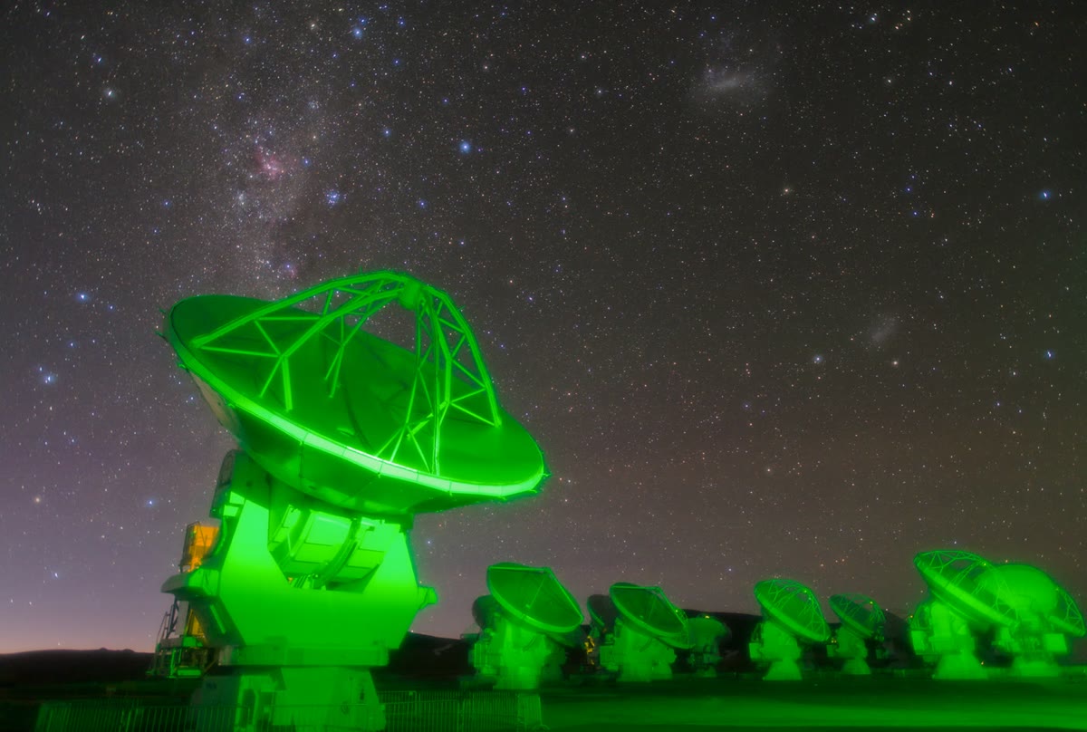
Antennas of a radio interferometer on a high plateau: they record, among many others, the rotational lines of carbon monoxide from interstellar clouds. Photograph ESO/B. Tafreshi (twanight.org), CC BY 4.0.

6.1 Rotational spectra

Definition 6.1 (Rotational constant, isotopologue)

The rotational constant of a linear molecule is $B = h/(8\pi^2cI)$ , in $\mathrm{cm}^{-1}$ (or $B = h/8\pi^2I$ in hertz), so that its rotational levels are $F(J) = BJ(J+1)$ in wavenumbers. Molecules that differ only in the isotopes of their atoms are isotopologues ( $\ce{^{12}C^{16}O}$ , $\ce{^{13}C^{16}O}$ ); in the Born–Oppenheimer approximation they share the same bond lengths and force constants.

Definition 6.2 (Gross and specific selection rules)

A gross selection rule states which property a molecule must have to show a kind of spectrum at all; a specific selection rule states which changes of quantum number are allowed.

Proposition 6.3 (Pure rotational spectra)

A molecule has a pure rotational (microwave) spectrum only if it has a permanent dipole moment; for a linear molecule the specific rule is $\Delta J = \pm1$ . Absorption lines lie at

\tilde\nu = F(J+1) - F(J) = 2B(J + 1), \qquad J = 0, 1, 2, \dots,

equally spaced by $2B$ .

Proof. The interaction with light is through the dipole moment: a molecule with no permanent dipole has no oscillating dipole when it rotates. The rule $\Delta J = \pm1$ comes from the vanishing of $\int Y_{J'M'}^*\cos\theta\,Y_{JM}$ unless $J' = J \pm 1$ (the dipole component along $z$ transforms like $Y_{1,0}$ ), admitted. Then $B(J+1)(J+2) - BJ(J+1) = 2B(J+1)$ . ∎

Method 6.4 (Bond length from a rotational line)

From the line $J + 1 \leftarrow J$ at frequency $\nu$ , deduce $B = \nu/2(J+1)$ (in hertz).
Compute the moment of inertia $I = h/8\pi^2B$ .
With the reduced mass from isotopic masses, $r = \sqrt{I/\mu}$ .

Example 6.5 (Carbon monoxide)

The line $J = 1 \leftarrow 0$ of $\ce{^{12}C^{16}O}$ is at $115\,271.20\,\mathrm{MHz}$ : $B = 57\,635.6\,\mathrm{MHz} = 1.922\,52\,\mathrm{cm}^{-1}$ , $I = 1.4560 \times 10^{-46}\,\mathrm{kg}\,\mathrm{m}^{2}$ . With $\mu = 12 \times 15.99491/27.99491 = 6.856\,21\,\mathrm{u}$ , $r_0 = 113.09\,\mathrm{pm}$ . This $r_0$ averages the bond over its zero-point vibration and is slightly longer than the equilibrium length $r_e$ (Section 6.2).

Definition 6.6 (Centrifugal distortion constant)

A rotating bond stretches; the levels become $F(J) = BJ(J+1) - DJ^2(J+1)^2$ , where $D$ is the centrifugal distortion constant, and the lines $2B(J+1) - 4D(J+1)^3$ close up slowly at high $J$ .

Proposition 6.7 (The strongest line)

If line intensities follow the population of the lower level, $(2J+1) \eu^{-hcBJ(J+1)/kT}$ , the most populated level is near

J_{\max} \approx \sqrt{\frac{kT}{2hcB}} - \frac12.

Proof. Treat $J$ as continuous and differentiate: $\frac{\dd}{\dd J}[(2J+1)\eu^{-aJ(J+1)}] = [2 - a(2J+1)^2]\eu^{-aJ(J+1)}$ with $a = hcB/kT$ ; it vanishes at $(2J + 1)^2 = 2/a$ . ∎

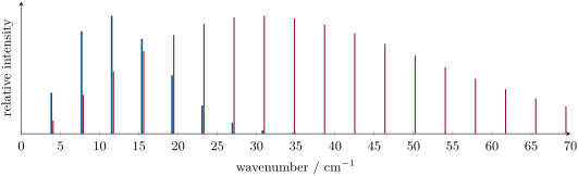
The rotational absorption spectrum of carbon monoxide, lines spaced by 2B = 3.845\, cm-1, intensities taken as the population of the lower level, at 30\, K (blue) and 300\, K (red, shifted slightly for visibility), each temperature scaled to its strongest line. At 30\, K the strongest line is J = 3 2; at 300\, K, J = 8 7. — The rotational absorption spectrum of carbon monoxide, lines spaced by $2B = 3.845\,\mathrm{cm}^{-1}$ , intensities taken as the population of the lower level, at $30\,\mathrm{K}$ (blue) and $300\,\mathrm{K}$ (red, shifted slightly for visibility), each temperature scaled to its strongest line. At $30\,\mathrm{K}$ the strongest line is $J = 3 \leftarrow 2$ ; at $300\,\mathrm{K}$ , $J = 8 \leftarrow 7$ .

6.2 Vibrations of real bonds

A real bond does not obey Hooke’s law far from equilibrium: it softens when stretched and breaks.

Definition 6.8 (Morse potential)

The Morse potential is $V(r) = D_e[1 - \eu^{-\beta(r - r_e)}]^2$ : harmonic near $r_e$ (force constant $2\beta^2D_e$ ), and tending to the dissociation limit $D_e$ at large $r$ .

Proposition 6.9 (Levels of the Morse oscillator)

In wavenumbers the vibrational levels of a Morse oscillator are

G(v) = \tilde\omega_e(v + \tfrac12) - \tilde\omega_ex_e(v + \tfrac12)^2, \qquad \tilde\omega_ex_e = \frac{\tilde\omega_e^2}{4D_e},

a ladder whose rungs close up and end at $v_{\max} = \lfloor\tilde\omega_e/ 2\tilde\omega_ex_e - \frac12\rfloor$ .

Proof. Admitted at this level. ∎

The solution of the Morse equation is treated in more advanced courses; the levels are checked numerically in this chapter’s figure data.

Definition 6.10 (Anharmonicity constant, fundamental, overtone, hot band)

$\tilde\omega_ex_e$ is the anharmonicity constant. The fundamental transition is $v = 1 \leftarrow 0$ ; an overtone is $v = n \leftarrow 0$ with $n \ge 2$ , weak because the gross rule $\Delta v = \pm1$ of the harmonic oscillator is only slightly broken; a hot band starts from an excited level, $v = 2 \leftarrow 1$ , and grows with temperature.

Definition 6.11 (Spectroscopic dissociation energy)

The spectroscopic dissociation energy of a molecule is the depth of its potential, $D_e$ , measured from the minimum, or $D_0 = D_e - G(0)$ , measured from the lowest level — per molecule at $0\,\mathrm{K}$ , unlike the bond dissociation enthalpy of the Year 2 volume, a molar enthalpy at $298\,\mathrm{K}$ .

Corollary 6.12 ( $D_e$ and $D_0$ of a Morse oscillator)

$D_e = \tilde\omega_e^2/4\tilde\omega_ex_e$ and $D_0 = D_e - (\frac12\tilde\omega_e - \frac14\tilde\omega_ex_e)$ .

Proof. The first is the relation of the proposition; the second is $G(0)$ . ∎

Proposition 6.13 (Birge–Sponer extrapolation)

The gaps $\Delta G(v + \frac12) = G(v+1) - G(v) = \tilde\omega_e - 2\tilde\omega_ex_e(v + 1)$ decrease linearly with $v$ ; summing them until they vanish gives $D_0$ , the area under the plot of $\Delta G$ against $v$ .

Proof. Subtract the two expressions of $G$ . $D_0$ is the energy from $v = 0$ to the limit, the sum of all the gaps. ∎

Example 6.14 (Hydrogen chloride)

For $\ce{H^{35}Cl}$ , $\tilde\omega_e = 2990.95\,\mathrm{cm}^{-1}$ and $\tilde\omega_ex_e = 52.82\,\mathrm{cm}^{-1}$ : the fundamental is at $\tilde\omega_e - 2\tilde\omega_ex_e = 2885.3\,\mathrm{cm}^{-1}$ and the first overtone at $2\tilde\omega_e - 6\tilde\omega_ex_e = 5665.0\,\mathrm{cm}^{-1}$ , slightly less than twice the fundamental. The Morse model predicts $D_e = 42\,342\,\mathrm{cm}^{-1}$ and $D_0 = 40\,860\,\mathrm{cm}^{-1}$ ; the true $D_0$ , from the enthalpies of formation of H, Cl and HCl at $0\,\mathrm{K}$ , is $35\,760\,\mathrm{cm}^{-1}$ ( $4.43\,\mathrm{eV}$ ). The real potential flattens out faster than a Morse curve fitted at the bottom: Birge–Sponer extrapolations from the lowest levels overestimate dissociation energies.

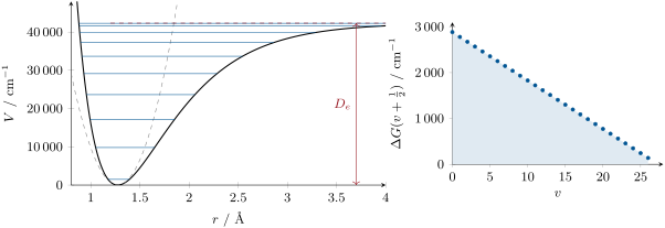
Left: the Morse potential of

\ce{HCl}

built from its spectroscopic constants (solid), the harmonic parabola with the same curvature (dashed), and every third vibrational level, drawn between its turning points; the levels close up towards

D_e

. Right: the Birge–Sponer plot of the gaps; the shaded area is

D_0

6.3 Rovibrational bands

A vibrational transition of a gas is accompanied by rotational changes, $\Delta J = \pm1$ for a diatomic in a ${}^1\Sigma$ state.

Definition 6.15 (P, Q and R branches, band origin)

In a rovibrational band, the lines with $\Delta J = -1$ form the P branch, those with $\Delta J = +1$ the R branch, and those with $\Delta J = 0$ , when allowed, the Q branch. The band origin $\tilde\nu_0$ is the vibrational energy difference without rotation.

Theorem 6.16 (Combination differences)

With rotational constants $B_0$ and $B_1$ in the lower and upper vibrational levels, $R(J) = \tilde\nu_0 + B_1(J+1)(J+2) - B_0J(J+1)$ and $P(J) = \tilde\nu_0 + B_1(J-1)J - B_0J(J+1)$ , and

R(J - 1) - P(J + 1) = 4B_0(J + \tfrac12), \qquad R(J) - P(J) = 4B_1(J + \tfrac12).

Proof. The first two follow from $E = G(v) + B_vJ(J+1)$ for both levels. $R(J - 1)$ and $P(J + 1)$ end on the same upper level $J$ , from lower levels $J - 1$ and $J + 1$ : their difference is $B_0[(J+1)(J+2) - (J-1)J] = B_0(4J + 2)$ . Likewise $R(J)$ and $P(J)$ start from the same lower level and end on $J + 1$ and $J - 1$ . ∎

Method 6.17 (Analysing a rovibrational band)

Locate the gap: for a ${}^1\Sigma$ diatomic there is no Q branch, and $\tilde\nu_0$ lies in the gap, between $R(0)$ and $P(1)$ .
Number the lines outwards from the gap: $R(0), R(1), \dots$ and $P(1), P(2), \dots$ .
Use the combination differences to get $B_0$ and $B_1$ separately, then $\alpha_e = B_0 - B_1$ and $B_e = B_0 + \frac12\alpha_e$ .

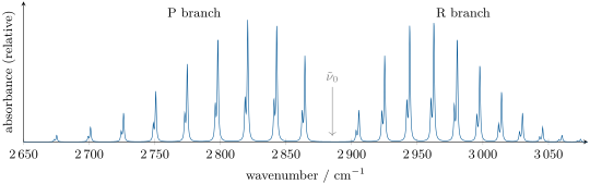
$The fundamental band of gaseous HCl at 300\, K, computed from its spectroscopic constants: P and R branches either side of the gap at the band origin. Each line is a doublet, H35Cl and the weaker, slightly lower H37Cl (natural abundances 76 % and 24 %). The R lines close up, the P lines spread out, because B_1 < B_0.$

The fundamental band of gaseous

\ce{HCl}

300\,\mathrm{K}

, computed from its spectroscopic constants: P and R branches either side of the gap at the band origin. Each line is a doublet,

\ce{H^{35}Cl}

and the weaker, slightly lower

\ce{H^{37}Cl}

(natural abundances 76 % and 24 %). The R lines close up, the P lines spread out, because

B_1 < B_0

Example 6.18 (The constants of $\ce{HCl}$ from its band)

With $R(0) = 2905.58\,\mathrm{cm}^{-1}$ and $P(2) = 2842.94\,\mathrm{cm}^{-1}$ , one finds $6B_0 = 62.64\,\mathrm{cm}^{-1}$ , so $B_0 = 10.440\,\mathrm{cm}^{-1}$ . With $R(1) = 2925.23$ and $P(1) = 2864.43\,\mathrm{cm}^{-1}$ , $B_1 = 10.133\,\mathrm{cm}^{-1}$ . So $\alpha_e = 0.307\,\mathrm{cm}^{-1}$ and $B_e = 10.593\,\mathrm{cm}^{-1}$ , the values the band was built from: the method recovers them exactly.

6.4 Raman spectroscopy

Definition 6.19 (Raman and Rayleigh scattering)

When light of frequency $\nu_0$ crosses a sample, most of the scattered light keeps the frequency $\nu_0$ : Rayleigh scattering. A small fraction is shifted by the rotational or vibrational frequencies of the molecules: Raman scattering. Lines at lower frequency are Stokes lines (the molecule gained energy), at higher frequency anti-Stokes lines (it lost energy).

Proposition 6.20 (Classical origin of the Raman effect)

If the polarisability of a molecule vibrating at $\nu_{\mathrm{vib}}$ varies as $\alpha = \alpha_0 + \alpha_1\cos(2\pi\nu_{\mathrm{vib}}t)$ , the dipole induced by a field $E_0\cos(2\pi\nu_0t)$ oscillates at $\nu_0$ and at $\nu_0 \pm \nu_{\mathrm{vib}}$ . A vibration is Raman active only if it changes the polarisability.

Proof. $\mu = \alpha E = \alpha_0E_0\cos(2\pi\nu_0t) + \frac12\alpha_1E_0[\cos2\pi(\nu_0 + \nu_{\mathrm{vib}})t + \cos2\pi(\nu_0 - \nu_{\mathrm{vib}})t]$ , by $\cos a\cos b = \frac12[\cos(a+b) + \cos(a-b)]$ . Each oscillating dipole radiates at its own frequency; without $\alpha_1$ only the Rayleigh term remains. ∎

Proposition 6.21 (Rotational Raman lines)

A linear molecule with an anisotropic polarisability shows rotational Raman lines with $\Delta J = \pm2$ , displaced from the exciting line by

|\Delta\tilde\nu| = F(J+2) - F(J) = 4B(J + \tfrac32) = 6B, 10B, 14B, \dots

— the first line at $6B$ , then a spacing of $4B$ .

Proof. The polarisability ellipsoid of a rotating linear molecule returns to the same orientation twice per turn, so it modulates the scattering at twice the rotation frequency: $\Delta J = \pm2$ (the quantum rule, admitted). Then $B(J+2)(J+3) - BJ(J+1) = B(4J + 6)$ . ∎

Example 6.22 (Nitrogen, seen by Raman)

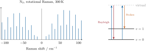
$\ce{N2}$ has no dipole and no infrared or microwave spectrum, but its polarisability is anisotropic: its rotational Raman lines start at $6B_0 = 11.94\,\mathrm{cm}^{-1}$ from the exciting line and are spaced by $7.96\,\mathrm{cm}^{-1}$ . Their intensities alternate 2:1 between even and odd $J$ : the two $\ce{^{14}N}$ nuclei are identical, and nuclear-spin statistics (Chapter 11) give even- $J$ levels twice the weight of odd ones.

Left: the rotational Raman spectrum of nitrogen computed at 300\, K: Stokes lines at positive shifts (right), anti-Stokes lines at negative shifts (left, slightly weaker), with the 2:1 alternation of intensities; the grey line at zero marks the much stronger Rayleigh line. Right: energy scheme of Rayleigh and Stokes scattering through a virtual level (not a real state of the molecule). — Left: the rotational Raman spectrum of nitrogen computed at $300\,\mathrm{K}$ : Stokes lines at positive shifts (right), anti-Stokes lines at negative shifts (left, slightly weaker), with the 2:1 alternation of intensities; the grey line at zero marks the much stronger Rayleigh line. Right: energy scheme of Rayleigh and Stokes scattering through a virtual level (not a real state of the molecule).

6.5 Polyatomic molecules

Definition 6.23 (Types of rotors)

A molecule with three equal principal moments of inertia is a spherical top ( $\ce{CH4}$ , $\ce{SF6}$ ); with two equal, a symmetric top ( $\ce{NH3}$ , $\ce{CHCl3}$ , $\ce{C6H6}$ ); with all three different, an asymmetric top ( $\ce{H2O}$ , most molecules); linear molecules have one moment zero.

A spherical top has no dipole and no rotational spectrum; a symmetric top has levels $BJ(J+1) + (A - B)K^2$ , where $K$ counts the angular momentum about its axis, and lines that still fall at $2B(J+1)$ since $\Delta K = 0$ ; an asymmetric top has an irregular spectrum, fitted by computer. The vibrations of polyatomic molecules are their normal modes, labelled and selected by Chapter 5: the infrared spectrum shows the modes that transform like $x$ , $y$ , $z$ , each with its own rotational structure.

In the lab — A gas cell in an infrared spectrometer

Gaseous $\ce{HCl}$ is admitted into a $10\,\mathrm{cm}$ cell with windows transparent in the infrared, inside a Fourier-transform spectrometer. At $1\,\mathrm{cm}^{-1}$ resolution the P and R branches appear as single lines; at $0.25\,\mathrm{cm}^{-1}$ each splits into its $\ce{H^{35}Cl}$ / $\ce{H^{37}Cl}$ doublet, $2\,\mathrm{cm}^{-1}$ apart. Hydrogen chloride is toxic and corrosive: the cell is filled on a vacuum line in a fume hood.

Safety

Hydrogen chloride gas: a gas under pressure, corrosive to skin, eyes and the respiratory tract, toxic if inhaled. Handled only in closed apparatus or a fume hood.

History — Raman, 1928

In 1928 C. V. Raman and K. S. Krishnan observed, in sunlight filtered through a violet filter and scattered by liquids, a faint light of different colour that a crossed green filter could isolate. Raman received the 1930 Nobel Prize in Physics; laser sources turned his effect into a routine analytical technique fifty years later.

6.6 Exercises

Exercise 6.1 ★

From $B_0 = 1.9225\,\mathrm{cm}^{-1}$ for $\ce{^{12}C^{16}O}$ , compute the moment of inertia and the bond length $r_0$ .

Solution

Solution of Exercise 6.1.

$I = h/(8\pi^2cB) = 6.62607 \times 10^{-34}/(8\pi^2 \times 2.99792 \times 10^{10} \times 1.9225) = 1.4561 \times 10^{-46}\,\mathrm{kg}\,\mathrm{m}^{2}$ . $\mu = 6.856\,21\,\mathrm{u} = 1.138\,50 \times 10^{-26}\,\mathrm{kg}$ , so $r_0 = \sqrt{I/\mu} = 113.09\,\mathrm{pm}$ .

Exercise 6.2 ★

With $B_0 = 10.440\,\mathrm{cm}^{-1}$ , give the positions of the first four lines of the rotational spectrum of $\ce{H^{35}Cl}$ and the $J$ of the strongest line at $300\,\mathrm{K}$ .

Solution

Solution of Exercise 6.2.

$2B_0(J+1)$ : 20.88, 41.76, 62.64, $83.52\,\mathrm{cm}^{-1}$ . $J_{\max} = \sqrt{kT/2hcB} - \frac12 = \sqrt{208.5/20.88} - 0.5 = 2.7$ : the level $J = 3$ is the most populated, and the strongest line is $4 \leftarrow 3$ at $83.5\,\mathrm{cm}^{-1}$ .

Exercise 6.3 ★

Which of $\ce{H2}$ , $\ce{HCl}$ , $\ce{N2}$ , $\ce{CO2}$ , $\ce{CH4}$ , $\ce{SF6}$ and $\ce{H2O}$ show a pure rotational absorption spectrum? A rotational Raman spectrum?

Solution

Solution of Exercise 6.3.

Microwave absorption needs a permanent dipole: $\ce{HCl}$ and $\ce{H2O}$ only. Rotational Raman needs an anisotropic polarisability: $\ce{H2}$ , $\ce{HCl}$ , $\ce{N2}$ , $\ce{CO2}$ , $\ce{H2O}$ ; not the spherical tops $\ce{CH4}$ and $\ce{SF6}$ .

Exercise 6.4 ★

What fraction of $\ce{HCl}$ molecules is in $v = 1$ at 300 and $1000\,\mathrm{K}$ (fundamental $2885.3\,\mathrm{cm}^{-1}$ )? When does the hot band become visible?

Solution

Solution of Exercise 6.4.

$N_1/N_0 = \eu^{-hc\tilde\nu/kT}$ : at $300\,\mathrm{K}$ , $\eu^{-13.84} = 9.8 \times 10^{-7}$ ; at $1000\,\mathrm{K}$ , $\eu^{-4.15} = 0.016$ . The hot band becomes noticeable (a per cent of the fundamental) only near $1000\,\mathrm{K}$ .

Exercise 6.5 ★★

The fundamental and first overtone of $\ce{H^{35}Cl}$ lie at 2885.3 and $5665.0\,\mathrm{cm}^{-1}$ . Deduce $\tilde\omega_e$ and $\tilde\omega_ex_e$ .

Solution

Solution of Exercise 6.5.

$\tilde\omega_e - 2\tilde\omega_ex_e = 2885.3$ and $2\tilde\omega_e - 6\tilde\omega_ex_e = 5665.0$ : subtracting twice the first from the second, $-2\tilde\omega_ex_e = -105.6$ , so $\tilde\omega_ex_e = 52.8\,\mathrm{cm}^{-1}$ and $\tilde\omega_e = 2990.9\,\mathrm{cm}^{-1}$ .

Exercise 6.6 ★★

With the constants of the previous exercise, compute $D_e$ and $D_0$ of the Morse model, and compare with the true $D_0 = 35\,760\,\mathrm{cm}^{-1}$ . Convert both $D_0$ into $\mathrm{kJ}/\mathrm{mol}$ .

Solution

Solution of Exercise 6.6.

$D_e = 2990.95^2/(4 \times 52.82) = 42\,341\,\mathrm{cm}^{-1}$ ; $G(0) = 1495.47 - 13.20 = 1482.3\,\mathrm{cm}^{-1}$ ; $D_0 = 40\,859\,\mathrm{cm}^{-1} = 488.8\,\mathrm{kJ}/\mathrm{mol}$ , against the true $35\,760\,\mathrm{cm}^{-1}$ $= 427.8\,\mathrm{kJ}/\mathrm{mol}$ : the Morse model overestimates by 14 %.

Exercise 6.7 ★★

Four lines of the $\ce{H^{35}Cl}$ fundamental are $R(0) = 2905.58$ , $R(1) = 2925.23$ , $P(1) = 2864.43$ and $P(2) = 2842.94\,\mathrm{cm}^{-1}$ . Find $B_0$ , $B_1$ , $\alpha_e$ and the band origin.

Solution

Solution of Exercise 6.7.

$R(0) - P(2) = 6B_0 = 62.64$ : $B_0 = 10.440\,\mathrm{cm}^{-1}$ . $R(1) - P(1) = 6B_1 = 60.80$ : $B_1 = 10.133\,\mathrm{cm}^{-1}$ . $\alpha_e = 0.307\,\mathrm{cm}^{-1}$ . $R(0) = \tilde\nu_0 + 2B_1$ gives $\tilde\nu_0 = 2885.31\,\mathrm{cm}^{-1}$ (and $P(1) = \tilde\nu_0 - 2B_0$ agrees).

Exercise 6.8 ★★

Predict $B_0$ and the band origin of $\ce{D^{35}Cl}$ from those of $\ce{H^{35}Cl}$ , using the reduced masses ( $\tilde\omega_e \propto \mu^{-1/2}$ , $\tilde\omega_ex_e \propto \mu^{-1}$ , $B \propto \mu^{-1}$ ).

Solution

Solution of Exercise 6.8.

$\mu_H = 0.979\,59\,\mathrm{u}$ , $\mu_D = 1.904\,41\,\mathrm{u}$ , $\mu_H/\mu_D = 0.51438$ . $B_0(\ce{DCl}) = 10.440 \times 0.51438 = 5.370\,\mathrm{cm}^{-1}$ . $\tilde\omega_e = 2990.95 \times \sqrt{0.51438} = 2145.1$ , $\tilde\omega_ex_e = 52.82 \times 0.51438 = 27.17$ : $\tilde\nu_0 = 2145.1 - 54.3 = 2090.8\,\mathrm{cm}^{-1}$ .

Exercise 6.9 ★★

For $\ce{N2}$ , $B_0 = 1.9896\,\mathrm{cm}^{-1}$ . Give the shifts of the first three Stokes rotational Raman lines, and explain the alternation of their intensities.

Solution

Solution of Exercise 6.9.

Shifts $4B_0(J + \frac32)$ : 11.94, 19.90, $27.85\,\mathrm{cm}^{-1}$ (from $J = 0$ , 1, 2). The two $\ce{^{14}N}$ nuclei are identical bosons of spin 1: the even- $J$ levels have six nuclear-spin states, the odd- $J$ three, so lines from even $J$ are twice as strong as their neighbours.

Exercise 6.10 ★★★

The first three rotational lines of $\ce{^{12}C^{16}O}$ are at 115271.2018, 230538.0000 and $345\,795.9899\,\mathrm{MHz}$ . Show that a rigid rotor does not fit them, and determine $B$ and the centrifugal distortion constant $D$ .

Solution

Solution of Exercise 6.10.

A rigid rotor would put the lines at $\nu_1$ , $2\nu_1$ , $3\nu_1$ : $230542.40$ and $345\,813.61\,\mathrm{MHz}$ , above the measured ones by 4.4 and $17.6\,\mathrm{MHz}$ . With $\nu_{J+1\leftarrow J} = 2B(J+1) - 4D(J+1)^3$ : $\nu_1 = 2B - 4D$ , $\nu_3 = 6B - 108D$ , so $3\nu_1 - \nu_3 = 96D$ : $D = 0.1835\,\mathrm{MHz}$ and $B = (\nu_1 + 4D)/2 = 57\,635.97\,\mathrm{MHz}$ . Check: $\nu_2 = 4B - 32D = 230\,538.0\,\mathrm{MHz}$ .

Exercise 6.11 ★★★

Show that the Birge–Sponer sum of the gaps $\Delta G(v + \frac12)$ of a Morse oscillator from $v = 0$ to the last bound level is close to $D_e - G(0)$ , and evaluate the sum for $\ce{HCl}$ .

Solution

Solution of Exercise 6.11.

$\Delta G(v + \frac12) = \tilde\omega_e - 2\tilde\omega_ex_e(v+1)$ vanishes near $v = \tilde\omega_e/2\tilde\omega_ex_e - 1$ ; the sum of an arithmetic progression of $n$ terms from $\tilde\omega_e - 2\tilde\omega_ex_e$ down to almost 0 is about $n\tilde\omega_e/2 \approx \tilde\omega_e^2/4\tilde\omega_ex_e - \tilde\omega_e/2 \approx D_e - G(0)$ . For $\ce{HCl}$ , the 28 gaps ( $v = 0$ to 27) add up to $40\,857\,\mathrm{cm}^{-1}$ , against $D_e - G(0) = 40\,859\,\mathrm{cm}^{-1}$ .

Exercise 6.12 ★★★

The $\ce{^{16}O}$ nucleus has spin zero, so the levels of $\ce{^{16}O^{12}C^{16}O}$ with odd $J$ do not exist. What is the spacing of its rotational Raman lines, and the shift of the first one, in terms of $B$ ? Why does $\ce{CO2}$ have no microwave spectrum?

Solution

Solution of Exercise 6.12.

With only even $J$ , the transitions $J \to J + 2$ start at $J = 0, 2, 4, \dots$ : shifts $6B, 14B, 22B, \dots$ , spacing $8B$ . $\ce{CO2}$ has a centre of symmetry and no permanent dipole: no microwave spectrum.

6.7 Problem: Listening to a Cold Cloud

Problem 6.1

Weekend problem — the bond length of carbon monoxide from its first rotational line, the temperature of an interstellar cloud, the carbon-13 isotopologue, and the infrared band

Data: $\ce{^{12}C^{16}O}$ lines $J = 1 \leftarrow 0$ at $115.2712\,\mathrm{GHz}$ and $2 \leftarrow 1$ at $230.5380\,\mathrm{GHz}$ ; $\ce{^{13}C^{16}O}$ line $1 \leftarrow 0$ at $110.2014\,\mathrm{GHz}$ ; masses $\ce{^{12}C}$ 12 (exactly), $\ce{^{13}C}$ 13.00335, $\ce{^{16}O}$ $15.994\,91\,\mathrm{u}$ ; natural abundance of $\ce{^{13}C}$ 1.1 %; for $\ce{^{12}C^{16}O}$ , $\tilde\omega_e = 2169.81\,\mathrm{cm}^{-1}$ , $\tilde\omega_ex_e = 13.288\,\mathrm{cm}^{-1}$ , and the equilibrium length $r_e = 112.83\,\mathrm{pm}$ . $h = 6.626\,07 \times 10^{-34}\,\mathrm{J}\,\mathrm{s}$ , $u = 1.660\,54 \times 10^{-27}\,\mathrm{kg}$ , $c = 2.997\,92 \times 10^{10}\,\mathrm{cm}/\mathrm{s}$ , $hc/k = 1.438\,78\,\mathrm{cm}\,\mathrm{K}$ .

Part I — The bond.

Compute $B_0$ in hertz and in $\mathrm{cm}^{-1}$ .
Compute the reduced mass of $\ce{^{12}C^{16}O}$ in kilograms.
Compute the moment of inertia.
Deduce $r_0$ .
Compare with $r_e$ . Why is $r_0$ longer?
Predict the $2 \leftarrow 1$ line for a rigid rotor. Comment on the measured value.

Part II — The temperature of the cloud.

Give the energies, in $\mathrm{cm}^{-1}$ and in kelvin ( $E/k$ ), of the levels $J = 0$ , 1, 2.
Write the ratio of the populations $N_2/N_1$ at temperature $T$ .
The observations give $N_2/N_1 = 0.85$ (data of the problem). Find $T$ .
Which level is the most populated at that temperature?
Why can such a cloud not be seen in the infrared vibrational band?
Why is the $1 \leftarrow 0$ line the most used tracer of cold gas?

Part III — The isotopologue.

Compute the reduced mass of $\ce{^{13}C^{16}O}$ .
Predict its $1 \leftarrow 0$ line from that of $\ce{^{12}C^{16}O}$ .
Compare with the measured $110.2014\,\mathrm{GHz}$ . What has been neglected?
If both lines were weak and unsaturated, what ratio of their intensities would the natural abundances give?
The observed ratio is far smaller. What does that say about the $\ce{^{12}C^{16}O}$ line?
Why are both isotopologues observed together in practice?

Part IV — The vibrational band.

Compute the band origin of the fundamental, in $\mathrm{cm}^{-1}$ and in micrometres.
Compute the first overtone.
Compute the zero-point energy.
What separates the first R and P lines?
Which molecule, $\ce{^{12}C^{16}O}$ or $\ce{^{13}C^{16}O}$ , has the lower band origin?
State the result: the bond length $r_0$ of carbon monoxide obtained from one radio line.

Solution

Solution of Problem 6.1.

1. $B_0 = \nu/2 = 57.6356\,\mathrm{GHz}$ ; $B_0/c = 1.922\,52\,\mathrm{cm}^{-1}$ . 2. $\mu = 12 \times 15.99491/27.99491 = 6.856\,21\,\mathrm{u} = 1.138\,50 \times 10^{-26}\,\mathrm{kg}$ . 3. $I = h/8\pi^2B_0 = 1.4560 \times 10^{-46}\,\mathrm{kg}\,\mathrm{m}^{2}$ . 4. $r_0 = \sqrt{I/\mu} = 113.09\,\mathrm{pm}$ . 5. $r_0$ exceeds $r_e = 112.83\,\mathrm{pm}$ by $0.26\,\mathrm{pm}$ : $B_0$ averages $1/r^2$ over the zero-point vibration in an anharmonic well, which spends more time at long distances. 6. $2\nu_{1\leftarrow0} = 230.5424\,\mathrm{GHz}$ ; the measured line is $4.4\,\mathrm{MHz}$ lower: centrifugal distortion. 7. $0$ , 3.845 and $11.535\,\mathrm{cm}^{-1}$ , i.e. $E/k = 0$ , 5.53 and $16.60\,\mathrm{K}$ . 8. $N_2/N_1 = \frac53\exp[-(16.60 - 5.53)\,\mathrm K/T]$ . 9. $\ln(\frac53/0.85) = 0.673 = 11.06/T$ : $T = 16\,\mathrm{K}$ . 10. $J_{\max} = \sqrt{16.4/(2 \times 1.43878 \times 1.9225)} - 0.5 = 1.2$ : $J = 1$ . 11. A vibrational quantum corresponds to $hc\tilde\nu/k \approx 3080\,\mathrm{K}$ : at $16\,\mathrm{K}$ no molecule is vibrationally excited, so the cloud emits no vibrational light. 12. It needs only $5.5\,\mathrm{K}$ of excitation, is excited even in the coldest gas, and CO is abundant and has a dipole moment. 13. $\mu = 13.00335 \times 15.99491/28.99826 = 7.172\,41\,\mathrm{u}$ . 14. $B \propto 1/\mu$ : $115.2712 \times 6.85621/7.17241 = 110.1893\,\mathrm{GHz}$ . 15. The prediction is $12\,\mathrm{MHz}$ (0.011 %) below the measured line: $B_0 = B_e - \frac12\alpha_e$ , and the vibration–rotation term $\alpha_e$ scales with a different power of $\mu$ ; the equilibrium structure is the same, the zero-point average is not. 16. $98.9/1.1 = 90$ . 17. The $\ce{^{12}C^{16}O}$ line is saturated (optically thick): it no longer grows with the amount of gas. 18. The rare $\ce{^{13}C^{16}O}$ line stays proportional to the amount of gas, the $\ce{^{12}C^{16}O}$ line gives the temperature: together they measure both. 19. $\tilde\nu_0 = 2169.81 - 2 \times 13.288 = 2143.24\,\mathrm{cm}^{-1}$ , $4.666\,\text{µ}\mathrm{m}$ . 20. $2\tilde\omega_e - 6\tilde\omega_ex_e = 4259.89\,\mathrm{cm}^{-1}$ . 21. $G(0) = \frac12\tilde\omega_e - \frac14\tilde\omega_ex_e = 1081.58\,\mathrm{cm}^{-1}$ . 22. $R(0) - P(1) = 2(B_0 + B_1) \approx 4B \approx 7.7\,\mathrm{cm}^{-1}$ . 23. $\ce{^{13}C^{16}O}$ : heavier reduced mass, lower frequency. 24. $r_0(\ce{CO}) = 113.1\,\mathrm{pm}$ , from a single radio frequency.

Terms defined in this chapter

See all 852 terms in the glossary