University Chemistry — Year 3 · Bachelor Year 3

32Environmental Chemistry and Toxicology

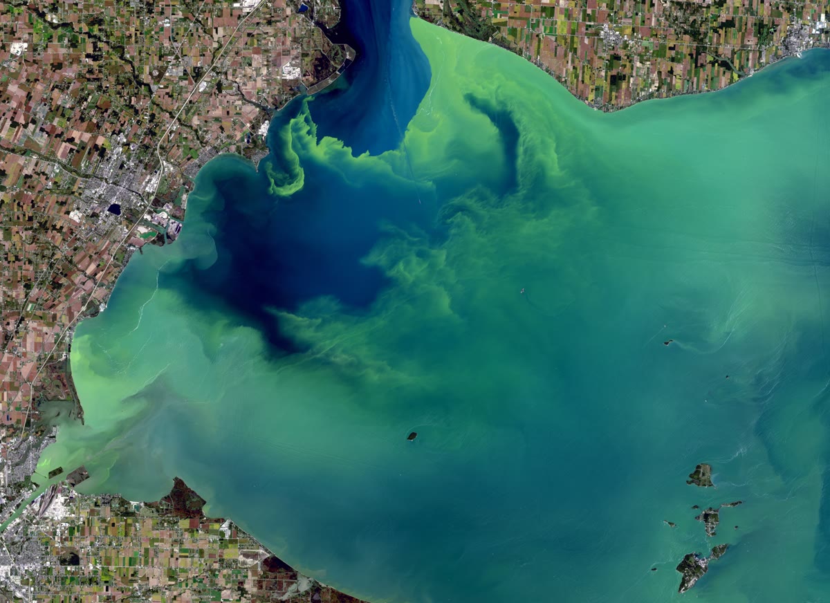
Every late summer, satellites photograph green swirls spreading over large lakes: blooms of algae fed by the phosphate and nitrate that run off fields and leave towns. When the algae die and sink, their decay uses up the oxygen of the deep water, and fish die. Chemistry explains each link of that chain, and of many others: why some gases warm the planet and others do not, why rain is acidic even in clean air, where a pesticide ends up once it is sprayed, and how much of a substance it takes to do harm. This chapter applies equilibria, kinetics and spectroscopy to the atmosphere, natural waters and soils, follows pollutants between them, and ends with the numbers on which risk assessments are built.

You already know

The Year 1 volume covered acid–base, precipitation and complexation equilibria, potential–pH diagrams, partition coefficients, half-lives, hazard, risk and the GHS system; the school volume greenhouse gases; the Year 2 volume Henry’s law, ionic strength, statistics, mass spectrometry and atomic spectrometry. Chapter 14 treated atmospheric photochemistry, Chapter 5 and Chapter 6 infrared activity, and Chapter 16 adsorption.

An algal bloom on a large lake, seen by an Earth-observation satellite in late September: the green swirls are dense populations of microscopic algae fed by nutrients from the farmland around. Image: USGS and NASA, public domain.

32.1 The atmosphere

Definition 32.1 (Greenhouse gases)

A greenhouse gas absorbs and emits infrared radiation at the wavelengths of the radiation emitted by the Earth’s surface, and so warms the lower atmosphere. The global warming potential (GWP) of a gas over a time horizon, usually 100 years, is the energy it traps after the emission of one kilogram, relative to one kilogram of carbon dioxide.

A molecule absorbs infrared radiation only through vibrations that change its dipole moment (Chapter 5). Dinitrogen and dioxygen, homonuclear diatomics, have no such vibration and are transparent; argon has no vibration at all. Carbon dioxide, linear and non-polar, has an infrared-active bending mode near $15\,\text{µ}\mathrm{m}$ , in the middle of the Earth’s emission; water, methane and nitrous oxide absorb at many wavelengths.

In 2025 the global mean mole fractions were $425.6\,\mathrm{ppm}$ of carbon dioxide, $1936\,\mathrm{ppb}$ of methane and $338.9\,\mathrm{ppb}$ of nitrous oxide. Methane, removed by hydroxyl radicals with a lifetime of about 12 years, has a GWP-100 of 27 to 30; nitrous oxide, destroyed only in the stratosphere with a lifetime of about 109 years, of 273. Carbon dioxide has no single lifetime: part of an emission stays in the air for centuries.

Definition 32.2 (Air pollutants)

Particulate matter is the solid and liquid particles suspended in air, classed by aerodynamic diameter (fine particles smaller than $2.5\,\text{µ}\mathrm{m}$ reach deep into the lungs). Acid rain is rain made more acidic than clean rain by sulfuric and nitric acids formed from sulfur dioxide and nitrogen oxides.

Proposition 32.3 (pH of clean rain)

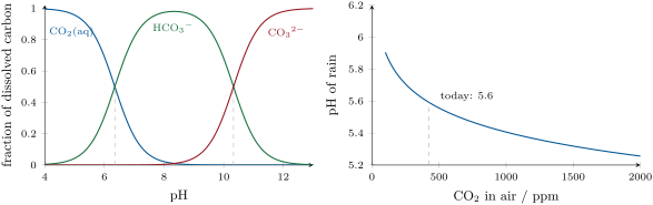
Rain in equilibrium with the carbon dioxide of today’s air, and with nothing else, has a pH of about 5.6.

Proof. Henry’s law gives $[\ce{CO2(aq)}] = K_Hp(\ce{CO2}) = 3.4 \times 10^{-7}\,\mathrm{mol}\,\mathrm{L}^{-1}\,\mathrm{Pa}^{-1} \times (425.6 \times 10^{-6} \times 101\,325\,\mathrm{Pa}) = 1.47 \times 10^{-5}\,\mathrm{mol}/\mathrm{L}$ . The charge balance is $[\ce{H+}] = [\ce{HCO3-}] + 2[\ce{CO3^2-}] + [\ce{OH-}] \approx K_{a1}[\ce{CO2(aq)}]/[\ce{H+}] + K_w/[\ce{H+}]$ , so $[\ce{H+}]^2 = K_{a1}[\ce{CO2(aq)}] + K_w = 10^{-6.35} \times 1.47 \times 10^{-5} + 10^{-14} = 6.6 \times 10^{-12}$ : $[\ce{H+}] = 2.6 \times 10^{-6}\,\mathrm{mol}/\mathrm{L}$ , pH 5.6. ∎

Sulfur dioxide from burning sulfur-containing fuel and nitrogen oxides from hot combustion are oxidised in the air, by hydroxyl radicals and in cloud droplets, to sulfuric and nitric acids, which bring rain down to pH 4 and below. Removing sulfur from fuels and nitrogen oxides from exhausts (catalytic converters, ammonia injection in power plants) has largely solved the problem where it was applied. Ozone near the ground, formed when sunlight acts on nitrogen oxides and volatile organic compounds (Chapter 14), and fine particles remain the main air pollutants for health.

32.2 Natural waters

Left: distribution of dissolved inorganic carbon among its three forms against pH at 25\, C, crossing at pK_a1 = 6.35 and pK_a2 = 10.33. Right: pH of rain in equilibrium with carbon dioxide alone, against its mole fraction in air. — Left: distribution of dissolved inorganic carbon among its three forms against pH at $25\,{}^{\circ}\mathrm{C}$ , crossing at $\mathrm pK_{a1} = 6.35$ and $\mathrm pK_{a2} = 10.33$ . Right: pH of rain in equilibrium with carbon dioxide alone, against its mole fraction in air.

Proposition 32.4 (Carbonate fractions)

With $C_T$ the total dissolved inorganic carbon, $[\ce{CO2(aq)}] = C_Th^2/D$ , $[\ce{HCO3-}] = C_TK_{a1}h/D$ , $[\ce{CO3^2-}] = C_TK_{a1}K_{a2}/D$ , where $h = [\ce{H+}]$ and $D = h^2 + K_{a1}h + K_{a1}K_{a2}$ .

Proof. From the two acidity constants,

[\ce{HCO3-}] = \frac{K_{a1}[\ce{CO2(aq)}]}{h}, \qquad [\ce{CO3^2-}] = \frac{K_{a2}[\ce{HCO3-}]}{h} = \frac{K_{a1}K_{a2}[\ce{CO2(aq)}]}{h^2}.

Their sum is $C_T = [\ce{CO2(aq)}]\,D/h^2$ ; dividing each form by $C_T$ gives the fractions. ∎

Definition 32.5 (Alkalinity)

The alkalinity of a water is its capacity to neutralise strong acid, measured by titration to the end point of carbonic acid (about pH 4.5) and expressed in moles of $\ce{H+}$ per litre.

Proposition 32.6 (Carbonate alkalinity)

In a water whose bases are carbonate species and hydroxide, $\mathrm{Alk} = [\ce{HCO3-}] + 2[\ce{CO3^2-}] + [\ce{OH-}] - [\ce{H+}]$ ; it equals the excess of the charges of the strong-base cations over those of the strong-acid anions, and does not change when carbon dioxide is exchanged with the air.

Proof. Titration to the carbonic acid end point turns every $\ce{HCO3-}$ into $\ce{CO2}$ (one $\ce{H+}$ each), every $\ce{CO3^2-}$ into $\ce{CO2}$ (two), every $\ce{OH-}$ into water (one), while the free $\ce{H+}$ already present counts against: the stated sum. The charge balance of the water, with $\ce{Na+}$ , $\ce{Ca^2+}$ … and $\ce{Cl-}$ , $\ce{SO4^2-}$ …, rearranges to the same sum equal to $\sum z_i c_i$ (cations) $-$ $\sum z_jc_j$ (anions) of the strong electrolytes. Adding or removing $\ce{CO2}$ changes none of these ions. ∎

Definition 32.7 (Ocean acidification)

Ocean acidification is the decrease of the pH of sea water as it takes up carbon dioxide from the air. The saturation state of a carbonate mineral is $\Omega = [\ce{Ca^2+}][\ce{CO3^2-}]/K_{sp}$ : above 1 the mineral can form, below 1 it tends to dissolve.

Dissolved carbon dioxide converts carbonate ions into hydrogencarbonate, $\ce{CO2 + CO3^2- + H2O -> 2HCO3-}$ , lowering the pH and $\Omega$ : shells and coral skeletons become harder to build. (In sea water the constants are apparent ones, measured in the salt medium, and differ from the fresh-water values of this chapter.)

Definition 32.8 (Water hardness)

The hardness of a water is its total concentration of calcium and magnesium ions, often expressed as the mass of calcium carbonate that would contain the same number of moles, in mg/L.

Definition 32.9 (Oxygen demand)

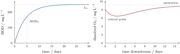
The biochemical oxygen demand (BOD) of a water is the mass of dioxygen consumed per litre by microorganisms oxidising its organic matter in the dark, over a stated time (five days at $20\,{}^{\circ}\mathrm{C}$ for $\mathrm{BOD_5}$ ). Its chemical oxygen demand (COD) is the mass of dioxygen equivalent to the dichromate consumed in oxidising its organic matter chemically.

Proposition 32.10 (BOD curve)

If biodegradable organic matter is consumed by first-order kinetics with rate constant $k$ , the oxygen used after time $t$ is $\mathrm{BOD}_t = L_0(1 - \eu^{-kt})$ , where $L_0$ is the ultimate BOD.

Proof. The remaining demand $L$ obeys $\dd L/\dd t = -kL$ , so $L = L_0\eu^{-kt}$ ; the oxygen used is what has gone, $L_0 - L$ . ∎

Left: the BOD of a model sewage, L_0 = 250\, mg/ L and k = 0.23\, d-1: about two thirds of the demand is used in five days. Right: the oxygen sag in a river below an outfall (Streeter–Phelps model): decay of the organic load consumes oxygen faster than the air restores it at first, until the deficit peaks after about 2.4 days. — Left: the BOD of a model sewage, $L_0 = 250\,\mathrm{mg}/\mathrm{L}$ and $k = 0.23\,\mathrm{d}^{-1}$ : about two thirds of the demand is used in five days. Right: the oxygen sag in a river below an outfall (Streeter–Phelps model): decay of the organic load consumes oxygen faster than the air restores it at first, until the deficit peaks after about 2.4 days.

Method 32.11 (Determining the COD)

Reflux a measured volume of sample with a known excess of potassium dichromate in sulfuric acid, with silver sulfate as catalyst and mercury(II) sulfate to bind chloride.
Titrate the remaining dichromate with iron(II) using ferroin, and run a blank with pure water.
The dichromate consumed, converted to the equivalent mass of $\ce{O2}$ (one $\ce{Cr2O7^2-}$ takes six electrons, as 1.5 $\ce{O2}$ would), divided by the sample volume, is the COD in mg/L.

Definition 32.12 (Eutrophication)

Eutrophication is the enrichment of a water body with nutrients, chiefly phosphorus and nitrogen, leading to excessive growth of algae and plants, then to oxygen depletion when they decay.

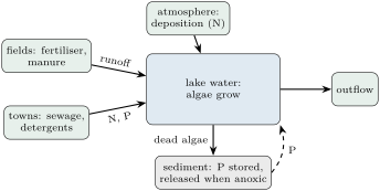
Nutrient flows into and within a lake. Phosphorus, often the limiting nutrient in fresh water, accumulates in the sediment and returns to the water when the bottom loses its oxygen, which can sustain blooms for years after the inputs are cut.

Algae take up carbon, nitrogen and phosphorus in roughly constant proportions; whichever nutrient is short relative to those needs limits their growth. In most lakes it is phosphorus, which is why phosphates were removed from detergents and from treated sewage; in many coastal seas it is nitrogen.

Definition 32.13 (Speciation)

The chemical speciation of an element in a sample is the distribution of its amount among its chemical forms: oxidation states, complexes, organometallic compounds, free and bound species.

Toxicity depends on speciation. Inorganic mercury released into water is methylated by bacteria in sediments into methylmercury, which crosses membranes, binds the sulfur of proteins and concentrates up food chains; arsenic is far more toxic as arsenite, As(III), than as arsenate, As(V), and much less so in the organic forms found in seafood. A total concentration alone says little.

Method 32.14 (Speciation of a metal in a water)

List the ligands present (hydroxide, carbonate, chloride, sulfate, organic matter) with their concentrations and the pH.
Write the complexation constants and the mass balance of the metal, as in the Year 1 volume.
Solve for the free metal ion, then each complex; draw the fractions against pH or against a ligand concentration.
Compare the toxic or bioavailable form (often the free ion) with the total.

32.3 Soils and sediments

Definition 32.15 (Sorption in soils)

The cation exchange capacity of a soil is the amount of exchangeable cations it can hold per unit mass, on clays and organic matter. The soil–water distribution coefficient $K_d$ is the ratio of the concentration of a substance sorbed on the soil (per kilogram) to its concentration in the pore water (per litre); the organic-carbon partition coefficient is $K_{oc} = K_d/f_{oc}$ , with $f_{oc}$ the mass fraction of organic carbon.

Neutral organic compounds sorb mainly on soil organic matter, so that $K_{oc}$ varies much less from soil to soil than $K_d$ . A compound with a small $K_d$ moves with water and can reach groundwater (leaching); one with a large $K_d$ stays near the surface, bound to particles that erosion may carry into rivers and lakes.

32.4 Fate of pollutants

Definition 32.16 (Octanol–water partition coefficient)

The octanol–water partition coefficient $K_{ow}$ of a substance is the ratio of its equilibrium concentrations in octan-1-ol and in water; it measures its affinity for fatty tissues and organic matter.

Benzene has $\log K_{ow} = 2.13$ , the herbicide atrazine 2.61, a hexachlorinated PCB 6.67 and DDT 6.91: the last two dissolve in fat tens of millions of times better than in water.

Definition 32.17 (Bioaccumulation)

The bioconcentration factor (BCF) is the ratio of the concentration in an organism to that in the surrounding water at steady state, uptake from water only. Bioaccumulation is the build-up in an organism from all routes, food included; biomagnification is the increase of concentration from prey to predator up a food chain.

Proposition 32.18 (BCF and $K_{ow}$ )

For neutral organic substances that are not metabolised, $\log\mathrm{BCF}$ in fish is approximately a linear function of $\log K_{ow}$ , with a slope close to 1, up to $\log K_{ow}$ near 6; above that, uptake slows and the relation levels off (empirical regressions).

Proof. Admitted at this level. ∎

Definition 32.19 (Persistent organic pollutants)

A persistent organic pollutant is an organic substance that resists degradation, bioaccumulates, is toxic and is transported far from its sources, such as DDT, the PCBs and the dioxins.

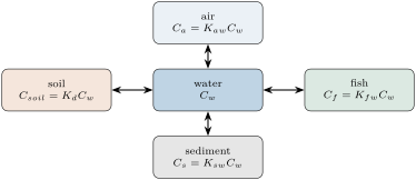
Proposition 32.20 (Equilibrium distribution between compartments)

A mass $M$ of a substance distributed at equilibrium (a “level I” model) among water (volume $V_w$ ), air ( $V_a$ ), sediment solids ( $m_s$ ) and fish ( $m_f$ ) has the water concentration $C_w = M/(V_w + K_{aw}V_a + K_{sw}m_s + K_{fw}m_f)$ , where the $K$ are the partition coefficients relative to water; the mass in each compartment is its term times $C_w$ .

Proof. At equilibrium $C_a = K_{aw}C_w$ , $C_s = K_{sw}C_w$ (per kilogram), $C_f = K_{fw}C_w$ . The mass balance is $M = C_wV_w + C_aV_a + C_sm_s + C_fm_f = C_w(V_w + K_{aw}V_a + K_{sw}m_s + K_{fw}m_f)$ ; dividing gives $C_w$ . ∎

Compartments of an equilibrium (level I) model: every compartment is in equilibrium with the water, its concentration fixed by a partition coefficient. The substance accumulates where the product of capacity and volume (or mass) is largest, often the sediment or soil for a hydrophobic compound.

32.5 Toxicology and regulation

Definition 32.21 (Dose–response)

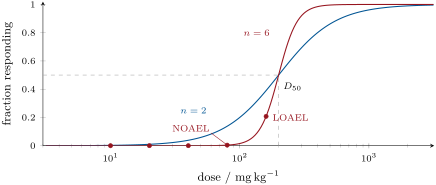
A dose–response relationship links the dose of a substance to the size or frequency of an effect. The median lethal dose $\mathrm{LD_{50}}$ kills half of a test population; the median effective concentration $\mathrm{EC_{50}}$ causes a stated effect in half. The no-observed-adverse-effect level (NOAEL) is the highest tested dose without an adverse effect, the lowest-observed-adverse-effect level (LOAEL) the lowest tested dose with one.

Proposition 32.22 (Log-logistic model)

In the log-logistic model $f(d) = 1/\bigl(1 + (D_{50}/d)^n\bigr)$ , the response is one half at $d = D_{50}$ , and $n$ measures the steepness: the dose ratio between 10 % and 90 % responses is $81^{1/n}$ .

Proof. At $d = D_{50}$ , $f = 1/2$ . $f = 0.1$ requires $(D_{50}/d)^n = 9$ , $f = 0.9$ requires $(D_{50}/d)^n = 1/9$ ; the ratio of the two doses is $(9 \times 9)^{1/n} = 81^{1/n}$ . ∎

Log-logistic dose–response curves with the same median dose (200\, mg/ kg, model) and two steepnesses. The dots are a study at five doses for the steeper curve: with a 5 % response as the criterion of an adverse effect, the NOAEL is 80\, mg/ kg and the LOAEL 160\, mg/ kg; both depend on the doses chosen. — Log-logistic dose–response curves with the same median dose ( $200\,\mathrm{mg}/\mathrm{kg}$ , model) and two steepnesses. The dots are a study at five doses for the steeper curve: with a 5 % response as the criterion of an adverse effect, the NOAEL is $80\,\mathrm{mg}/\mathrm{kg}$ and the LOAEL $160\,\mathrm{mg}/\mathrm{kg}$ ; both depend on the doses chosen.

Definition 32.23 (Acute and chronic toxicity)

Acute toxicity is the harm caused by a single exposure or exposures within a short time; chronic toxicity, by repeated or continuous exposure over a long part of a lifetime.

Toxicity is a matter of dose: the oral $\mathrm{LD_{50}}$ in rats is about $3000\,\mathrm{mg}/\mathrm{kg}$ for sodium chloride, $192\,\mathrm{mg}/\mathrm{kg}$ for caffeine and $188\,\mathrm{mg}/\mathrm{kg}$ for nicotine in the same kind of record. For most effects a threshold dose exists below which the body copes; for genotoxic carcinogens none is assumed, and exposure is kept as low as reasonably achievable.

Definition 32.24 (Ecotoxicology)

Ecotoxicology studies the effects of substances on organisms in ecosystems. The predicted no-effect concentration (PNEC) is the lowest effect or no-effect concentration from tests on representative species, divided by an assessment factor that covers the uncertainty; the predicted environmental concentration (PEC) is the concentration expected from the uses and fate of the substance; the risk quotient is PEC/PNEC.

Proposition 32.25 (Risk quotient)

A risk quotient below 1 indicates no concern for the compartment assessed; above 1, a risk that calls for refined data or measures to reduce exposure.

By definition. The PNEC is set, through its assessment factor, below the concentrations at which effects were seen; an expected concentration below it is therefore not expected to cause effects, and above it is. ∎

Method 32.26 (An environmental risk assessment)

Hazard: collect toxicity data for algae, invertebrates and fish (acute $\mathrm{EC_{50}}$ , chronic NOEC); take the lowest; divide by the assessment factor (larger when only acute data exist) to get the PNEC.
Exposure: from the amounts used and the fate (partitioning, degradation), compute the PEC in each compartment, or measure it.
Risk: compute PEC/PNEC; if above 1, refine the data or reduce the exposure, and repeat.

Definition 32.27 (Occupational exposure limit)

An occupational exposure limit is the concentration of a substance in the air of a workplace that workers may breathe, averaged over a working day (or over 15 minutes for short-term limits), without expected adverse effects.

New chemicals placed on a market in quantity must be registered with a dossier of their properties, hazards and uses; the most hazardous may be restricted or allowed only for authorised uses.

In the lab — Measuring $\mathrm{BOD_5}$

A sample is diluted with aerated dilution water containing nutrients and a bacterial seed, so that a good part, but not all, of the oxygen will be consumed. Two stoppered bottles are filled to the brim: the dissolved oxygen of one is measured at once with an oxygen electrode, the other after five days in the dark at $20\,{}^{\circ}\mathrm{C}$ . The difference, times the dilution factor and corrected for the seed, is the $\mathrm{BOD_5}$ .

Safety

The COD reagents: potassium dichromate is an oxidiser, may cause cancer and genetic defects, is corrosive and sensitising; mercury(II) sulfate is fatal if swallowed, inhaled or in contact with skin and very toxic to aquatic life. Both are used in sealed tubes, and the spent tubes go to hazardous waste.

History — A book and a bay

In 1962 Rachel Carson’s Silent Spring described the decline of birds poisoned by DDT and other pesticides concentrated up food chains, and launched modern environmental regulation. A few years earlier, in 1956, a disease of the nervous system was recognised among the people of Minamata Bay: a chemical plant had discharged methylmercury, formed from its mercury catalyst, which accumulated in the fish the inhabitants ate.

32.6 Exercises

Exercise 32.1 ★

Why do $\ce{N2}$ , $\ce{O2}$ and Ar not absorb in the infrared, and which vibration of $\ce{CO2}$ makes it a greenhouse gas?

Solution

Solution of Exercise 32.1.

A homonuclear diatomic has a single vibration that keeps the dipole moment zero, and argon has no vibration: none can absorb infrared radiation. $\ce{CO2}$ absorbs through its bending mode (and its antisymmetric stretch), which create an oscillating dipole; the bend lies in the middle of the Earth’s emission.

Exercise 32.2 ★

By what factor does $[\ce{H+}]$ change when the pH of sea water falls by 0.1?

Solution

Solution of Exercise 32.2.

$10^{0.1} = 1.26$ : $[\ce{H+}]$ rises by 26 %.

Exercise 32.3 ★

A water contains $2.0\,\mathrm{mmol}/\mathrm{L}$ of $\ce{Ca^2+}$ and $0.50\,\mathrm{mmol}/\mathrm{L}$ of $\ce{Mg^2+}$ . Give its hardness in mg of $\ce{CaCO3}$ per litre.

Solution

Solution of Exercise 32.3.

$(2.0 + 0.50)\ \mathrm{mmol}/\mathrm{L} \times 100.1\,\mathrm{mg}/\mathrm{mmol} = 250\,\mathrm{mg}/\mathrm{L}$ of $\ce{CaCO3}$ .

Exercise 32.4 ★

Algae take up C, N and P in the mole ratio $106 : 16 : 1$ (data of the exercise). A lake water has $0.60\,\mathrm{mg}/\mathrm{L}$ of nitrate nitrogen and $0.010\,\mathrm{mg}/\mathrm{L}$ of phosphate phosphorus. Which nutrient limits growth?

Solution

Solution of Exercise 32.4.

N: $0.60/14.0 = 0.043\,\mathrm{mmol}/\mathrm{L}$ ; P: $0.010/31.0 = 3.2 \times 10^{-4}\,\mathrm{mmol}/\mathrm{L}$ ; N : P $= 133$ , far above 16: phosphorus runs out first and limits growth.

Exercise 32.5 ★★

A $\mathrm{BOD_5}$ of $170\,\mathrm{mg}/\mathrm{L}$ is measured on a sewage with $k = 0.23\,\mathrm{d}^{-1}$ . Estimate its ultimate BOD.

Solution

Solution of Exercise 32.5.

$L_0 = \mathrm{BOD_5}/(1 - \eu^{-0.23 \times 5}) = 170/0.683 = 250\,\mathrm{mg}/\mathrm{L}$ .

Exercise 32.6 ★★

A $100.0\,\mathrm{mL}$ water sample needs $4.40\,\mathrm{mL}$ of $0.0200\,\mathrm{mol}/\mathrm{L}$ hydrochloric acid to reach pH 4.5. Compute its alkalinity and, assuming it is all hydrogencarbonate, its concentration in mg/L.

Solution

Solution of Exercise 32.6.

$4.40 \times 10^{-3}\,\mathrm{L} \times 0.0200\,\mathrm{mol}/\mathrm{L} = 8.80 \times 10^{-5}\,\mathrm{mol}$ in $0.1000\,\mathrm{L}$ : alkalinity $8.80 \times 10^{-4}\,\mathrm{mol}/\mathrm{L}$ ; as $\ce{HCO3-}$ ( $61.0\,\mathrm{g}/\mathrm{mol}$ ), $53.7\,\mathrm{mg}/\mathrm{L}$ .

Exercise 32.7 ★★

A soil has $f_{oc} = 0.020$ ; a pesticide has $K_{oc} = 300\,\mathrm{L}/\mathrm{kg}$ (data of the exercise). Compute $K_d$ and the fraction of the pesticide sorbed in a soil with $1.5\,\mathrm{kg}$ of solid per $0.30\,\mathrm{L}$ of pore water.

Solution

Solution of Exercise 32.7.

$K_d = 0.020 \times 300 = 6.0\,\mathrm{L}/\mathrm{kg}$ . Sorbed/total $= K_dm_s/(K_dm_s + V_w) = 9.0/(9.0 + 0.30) = 0.97$ : 97 % sorbed.

Exercise 32.8 ★★

With $\log\mathrm{BCF} = 0.85\log K_{ow} - 0.70$ (an empirical regression, data of the exercise), estimate the BCF of benzene and of a hexachlorinated PCB, and comment.

Solution

Solution of Exercise 32.8.

Benzene: $\log\mathrm{BCF} = 0.85 \times 2.13 - 0.70 = 1.11$ , BCF about 13. PCB: $0.85 \times 6.67 - 0.70 = 4.97$ , BCF about $9 \times 10^{4}$ : it concentrates in fish some seven thousand times more than benzene; at such $K_{ow}$ the regression is near its limit of validity.

Exercise 32.9 ★★

Express the rat oral $\mathrm{LD_{50}}$ of caffeine as a mass for a $70\,\mathrm{kg}$ adult and as cups of coffee of $90\,\mathrm{mg}$ each (a naive scaling, data of the exercise). Why is such a scaling only indicative?

Solution

Solution of Exercise 32.9.

$192\,\mathrm{mg}/\mathrm{kg} \times 70\,\mathrm{kg} = 13\,\mathrm{g}$ , about 150 cups. Species differ in absorption and metabolism, and an $\mathrm{LD_{50}}$ is not a safe threshold; harmful effects begin far below it.

Exercise 32.10 ★★★

A substance has a 48-hour $\mathrm{EC_{50}}$ of $0.50\,\mathrm{mg}/\mathrm{L}$ for water fleas, a 72-hour $\mathrm{EC_{50}}$ of $1.2\,\mathrm{mg}/\mathrm{L}$ for algae and a 96-hour $\mathrm{LC_{50}}$ of $2.0\,\mathrm{mg}/\mathrm{L}$ for fish, all acute, and an assessment factor of 1000 applies (data of the exercise). Compute the PNEC, and the risk quotient for a PEC of $0.20\,\text{µ}\mathrm{g}/\mathrm{L}$ .

Solution

Solution of Exercise 32.10.

PNEC $= 0.50\,\mathrm{mg}/\mathrm{L}/1000 = 0.50\,\text{µ}\mathrm{g}/\mathrm{L}$ ; $\mathrm{RQ} = 0.20/0.50 = 0.40$ , below 1: no concern at this exposure.

Exercise 32.11 ★★★

A fish-eating bird eats fish with $0.30\,\mathrm{mg}/\mathrm{kg}$ of a persistent pollutant; the fish eat plankton with $0.015\,\mathrm{mg}/\mathrm{kg}$ ; the water contains $2.0\,\mathrm{ng}/\mathrm{L}$ . Compute the bioconcentration and biomagnification factors along the chain if the bird’s fat holds $6.0\,\mathrm{mg}/\mathrm{kg}$ (data of the exercise).

Solution

Solution of Exercise 32.11.

Plankton/water: $0.015\,\mathrm{mg}/\mathrm{kg}/2.0 \times 10^{-6}\,\mathrm{mg}/\mathrm{L} = 7.5 \times 10^{3}\,\mathrm{L}/\mathrm{kg}$ (bioconcentration). Fish/plankton: $0.30/0.015 = 20$ ; bird/fish: $6.0/0.30 = 20$ (biomagnification at each step); bird/water: $3 \times 10^{6}$ .

Exercise 32.12 ★★★

A power plant emits $1000\,\mathrm{t}$ of $\ce{SO2}$ a year. Compute the mass of sulfuric acid it can make, and the volume of rain it would bring to pH 4.0 if all of it fell in rain (ignore other acids and bases).

Solution

Solution of Exercise 32.12.

$1.0 \times 10^{9}\,\mathrm{g}/64.1\,\mathrm{g}/\mathrm{mol} = 1.56 \times 10^{7}\,\mathrm{mol}$ of $\ce{SO2}$ , giving as many moles of $\ce{H2SO4}$ : $1.53 \times 10^{9}\,\mathrm{g}$ , about $1500\,\mathrm{t}$ . It releases $3.12 \times 10^{7}\,\mathrm{mol}$ of $\ce{H+}$ ; at pH 4.0, $[\ce{H+}] = 1.0 \times 10^{-4}\,\mathrm{mol}/\mathrm{L}$ : $3.1 \times 10^{11}\,\mathrm{L}$ of rain.

32.7 Problem: A Pesticide in a Lake

Problem 32.1

Weekend problem — a pesticide in a lake: its partitioning into sediment and fish, an equilibrium mass balance, its degradation over a year, and the risk quotient for the lake’s organisms

Data of the problem. A lake holds $1.0 \times 10^{9}\,\mathrm{L}$ of water under $1.0 \times 10^{12}\,\mathrm{L}$ of air (the mixed layer above it), with $1.0 \times 10^{8}\,\mathrm{kg}$ of active sediment solids ( $f_{oc} = 0.040$ ) and $1.0 \times 10^{4}\,\mathrm{kg}$ of fish (lipid fraction 0.048). A pesticide has $\log K_{ow} = 4.0$ , an air–water partition coefficient $K_{aw} = 1.0 \times 10^{-4}$ , and $K_{oc} = 0.41\,K_{ow}$ ; $K_{fw}$ = lipid fraction $\times K_{ow}$ . 100 kg of it reach the lake. Its half-life in the lake is 60 days. The most sensitive chronic test gives a NOEC of $50\,\text{µ}\mathrm{g}/\mathrm{L}$ , with an assessment factor of 10; fish for human consumption should not exceed $1.0\,\mathrm{mg}/\mathrm{kg}$ .

Part I — Partition coefficients.

What does $\log K_{ow} = 4.0$ say about the pesticide?
Compute $K_{oc}$ and the sediment–water coefficient $K_{sw}$ .
Compute the fish–water coefficient $K_{fw}$ .
Is the pesticide volatile from water? Use $K_{aw}$ .
Why does organic carbon, not mineral matter, govern its sorption?
Which compartment do you expect to hold most of it?

Part II — Equilibrium mass balance.

Compute the capacity terms $V_w$ , $K_{aw}V_a$ , $K_{sw}m_s$ and $K_{fw}m_f$ .
Compute the water concentration.
Compute the mass in each compartment.
Compute the concentrations in air, sediment and fish.
Which assumption of the model is least realistic?
How would degradation change the picture (level II and III models)?

Part III — Degradation.

Compute the first-order rate constant.
Compute the fraction left after one year.
Compute the water concentration after one year.
Why may the sediment hold the pesticide longer than the half-life suggests?
What makes a pesticide persistent?

Part IV — Risk.

Compute the PNEC.
Take the initial water concentration as PEC: compute the risk quotient.
Conclude for the lake’s organisms.
Compare the fish concentration with the consumption threshold.
What would you measure next, and where?
Which measures would lower the PEC?
Why does the assessment factor matter so much?
State the result: the risk quotient PEC/PNEC.

Solution

Solution of Problem 32.1.

1. It is ten thousand times more soluble in octanol than in water: hydrophobic, it will sorb on organic matter and accumulate in fat.

2. $K_{oc} = 0.41 \times 10^4 = 4100\,\mathrm{L}/\mathrm{kg}$ ; $K_{sw} = f_{oc}K_{oc} = 0.040 \times 4100 = 164\,\mathrm{L}/\mathrm{kg}$ .

3. $K_{fw} = 0.048 \times 10^4 = 480\,\mathrm{L}/\mathrm{kg}$ .

4. No: at equilibrium the air holds $10^{-4}$ of the water concentration.

5. The neutral, hydrophobic molecule dissolves in the organic matter, as in octanol; mineral surfaces are polar and covered with water.

6. The sediment, whose capacity, $K_{sw}m_s$ , is largest.

7. $V_w = 1.0 \times 10^{9}\,\mathrm{L}$ ; $K_{aw}V_a = 1.0 \times 10^{8}\,\mathrm{L}$ ; $K_{sw}m_s = 1.64 \times 10^{10}\,\mathrm{L}$ ; $K_{fw}m_f = 4.8 \times 10^{6}\,\mathrm{L}$ .

8. $C_w = 1.0 \times 10^{8}\,\mathrm{mg}/1.75 \times 10^{10}\,\mathrm{L} = 5.7 \times 10^{-3}\,\mathrm{mg}/\mathrm{L}$ , $5.7\,\text{µ}\mathrm{g}/\mathrm{L}$ .

9. Water $5.7\,\mathrm{kg}$ , air $0.57\,\mathrm{kg}$ , sediment $94\,\mathrm{kg}$ , fish $0.027\,\mathrm{kg}$ .

10. Air $5.7 \times 10^{-7}\,\mathrm{mg}/\mathrm{L}$ ; sediment $0.94\,\mathrm{mg}/\mathrm{kg}$ ; fish $2.7\,\mathrm{mg}/\mathrm{kg}$ .

11. Equilibrium between all compartments at once, with no degradation, no inflow or outflow, and well-mixed compartments.

12. With degradation and flows at steady state (level II) the inventory is set by the rates of input and loss; with transfer rates between compartments (level III) the concentrations are no longer in equilibrium ratios, and the compartment that receives the input is enriched.

13. $k = \ln 2/60\,\mathrm{d} = 0.0116\,\mathrm{d}^{-1}$ .

14. $\eu^{-0.0116 \times 365} = 0.0145$ : 1.5 % left.

15. $5.7\,\text{µ}\mathrm{g}/\mathrm{L} \times 0.0145 = 0.083\,\text{µ}\mathrm{g}/\mathrm{L}$ .

16. Degradation is often slower in cold, anoxic sediment, and the sorbed pesticide is released back to the water slowly, keeping it present after the water has been cleared.

17. Bonds that resist hydrolysis, oxidation and microbial attack (aromatic C–Cl, for example), low water solubility, and sorption that protects it from degraders.

18. PNEC $= 50\,\text{µ}\mathrm{g}/\mathrm{L}/10 = 5.0\,\text{µ}\mathrm{g}/\mathrm{L}$ .

19. $\mathrm{RQ} = 5.7/5.0 = 1.1$ .

20. Just above 1: a risk is indicated, and the assessment must be refined (better toxicity data, measured concentrations) or the exposure reduced.

21. $2.7\,\mathrm{mg}/\mathrm{kg}$ , almost three times the $1.0\,\mathrm{mg}/\mathrm{kg}$ threshold: the fish should not be eaten until the concentration falls.

22. Concentrations in water, sediment and fish over time and at several points, to check the model and follow the decline.

23. Less pesticide applied, application away from rain and from the shore, buffer strips that hold runoff, or a less persistent alternative.

24. It divides the measured no-effect level to cover the gap between a few laboratory species and a whole ecosystem; a factor of 10 instead of 1000 changes the PNEC, and the verdict, a hundredfold.

25. The risk quotient PEC/PNEC is about 1.1, just above 1.

Terms defined in this chapter

See all 852 terms in the glossary