Primary & Middle School Mathematics · Grades 1–9

71Statistics and Probability

Data and chance are everywhere: sports results, weather forecasts, games. This chapter teaches how to summarize a series of numbers by its mean, median and range, and how to compute the probability of simple random experiments — including two-step experiments, handled with tree diagrams. Both subjects are developed much further in the High School volume of this series.

71.1 Summarizing data

Definition 71.1 (Mean, median, range)

For a series of $N$ numbers:

the mean is the sum of all the values divided by $N$ ;
the median is a value splitting the sorted series in two halves of equal size: for $N$ odd, the middle value; for $N$ even, the midpoint of the two middle values;
the range is the largest value minus the smallest.

Example 71.2

Marks of a student: $8,\ 12,\ 9,\ 15,\ 11$ .

Mean: $\dfrac{8 + 12 + 9 + 15 + 11}{5} = \dfrac{55}{5} = 11$ .
Median: sort the series: $8, 9, 11, 12, 15$ ; the middle (3rd) value is $11$ .
Range: $15 - 8 = 7$ .

With a sixth mark of $17$ : sorted $8, 9, 11, 12, 15, 17$ , the median becomes the midpoint of $11$ and $12$ , that is $11.5$ , and the mean becomes $\frac{72}{6} = 12$ .

Example 71.3 (Weighted mean)

The shoe sizes sold in a day:

size	$38$	$39$	$40$	$41$	$42$
count	$3$	$7$	$6$	$3$	$1$

The mean size is

\frac{3 \times 38 + 7 \times 39 + 6 \times 40 + 3 \times 41 + 1 \times 42} {3 + 7 + 6 + 3 + 1} = \frac{114 + 273 + 240 + 123 + 42}{20} = \frac{792}{20} = 39.6 .

Remark 71.4

The mean and the median can differ a lot. In the series $10, 10, 10, 10, 60$ the mean is $20$ (pulled up by the value $60$ ) while the median is $10$ . Always ask which indicator represents the situation better.

71.2 Probability

Definition 71.5 (Probability)

A random experiment has several possible outcomes; an event is a set of outcomes. Each outcome gets a probability: a number between $0$ and $1$ , with all the probabilities of the outcomes summing to $1$ ; the probability $\P(A)$ of an event $A$ is the sum of the probabilities of its outcomes. When all $n$ outcomes are equally likely,

\P(A) = \frac{\text{number of favorable outcomes}}{n}.

Example 71.6

A wheel is split into $8$ equal sectors: $3$ red, $3$ blue, $2$ green. Each sector has probability $\frac18$ , so

\P(\text{red}) = \frac38, \qquad \P(\text{green}) = \frac28 = \frac14, \qquad \P(\text{not green}) = 1 - \frac14 = \frac34 .

Proposition 71.7 (Complement)

For every event $A$ , the contrary event $\bar A$ (“ $A$ does not occur”) satisfies

\P(\bar A) = 1 - \P(A).

Proof. Every outcome is in exactly one of $A$ and $\bar A$ , so $\P(A) + \P(\bar A)$ sums the probabilities of all outcomes, which is $1$ . ∎

71.3 Two-step experiments

Method 71.8 (Tree diagrams)

For an experiment in two steps:

draw one branch per outcome of the first step, then continue each branch with the outcomes of the second step, writing each probability on its branch;
multiply the probabilities along a path to get the probability of that path;
add the probabilities of all the paths forming an event.

Example 71.9

A bag holds $2$ red and $3$ black tokens. Draw one token, note its color, put it back, draw again. Each draw gives red with probability $\frac25$ , black with probability $\frac35$ .

The tree of the two draws with replacement: multiply along the branches, and check that the four paths sum to 1. — The tree of the two draws with replacement: multiply along the branches, and check that the four paths sum to $1$ .

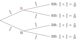
Probability of two tokens of the same color: $\frac{4}{25} + \frac{9}{25} = \frac{13}{25}$ . Probability of at least one red: $1 - \P(\text{BB}) = 1 - \frac{9}{25} = \frac{16}{25}$ .

Remark 71.10 (Frequencies approach probabilities)

Rolling a fair die $6000$ times gives about $1000$ sixes — not exactly. As the number of repetitions grows, observed frequencies get closer and closer to the probabilities: this is what makes probability the right tool to model repeated experiments (a story developed in the High School volume of this series).

71.4 Exercises

Exercise 71.1 ★

Compute the mean, median and range of the series $14,\ 9,\ 17,\ 9,\ 12,\ 11,\ 12$ .

Solution

Solution of Exercise 71.1.

Mean: $\dfrac{14 + 9 + 17 + 9 + 12 + 11 + 12}{7} = \dfrac{84}{7} = 12$ .

Median: sorted, $9, 9, 11, 12, 12, 14, 17$ ; the middle ( $4$ th) value is $12$ .

Range: $17 - 9 = 8$ .

Exercise 71.2 ★

The temperatures at noon over a week were $19,\ 21,\ 24,\ 18,\ 22,\ 25,\ 19$ (degrees). Compute the mean (to a tenth) and the median.

Solution

Solution of Exercise 71.2.

Mean: $\dfrac{19 + 21 + 24 + 18 + 22 + 25 + 19}{7} = \dfrac{148}{7} \approx 21.1$ degrees.

Median: sorted, $18, 19, 19, 21, 22, 24, 25$ ; the $4$ th value is $21$ degrees.

Exercise 71.3 ★

The number of goals scored by a team in $10$ matches:

goals	$0$	$1$	$2$	$3$
matches	$2$	$4$	$3$	$1$

Compute the mean number of goals per match, and the median.

Solution

Solution of Exercise 71.3.

Mean:

\frac{2 \times 0 + 4 \times 1 + 3 \times 2 + 1 \times 3}{10} = \frac{0 + 4 + 6 + 3}{10} = \frac{13}{10} = 1.3 \text{ goals per match.}

Median: the sorted series is $0,0,1,1,1,1,2,2,2,3$ ; the $5$ th and $6$ th values are both $1$ : median $1$ .

Exercise 71.4 ★

A fair die is rolled once. Compute the probability of: “rolling a $3$ ”; “rolling an even number”; “rolling at least a $3$ ”; “not rolling a $6$ ”.

Solution

Solution of Exercise 71.4.

$\P(3) = \frac16$ . $\P(\text{even}) = \frac36 = \frac12$ . $\P(\text{at least } 3) = \P(\{3,4,5,6\}) = \frac46 = \frac23$ . $\P(\text{not } 6) = 1 - \frac16 = \frac56$ .

Exercise 71.5 ★

A box contains $12$ balls: $5$ white, $4$ red and $3$ green; one ball is drawn at random. Compute $\P(\text{white})$ , $\P(\text{red or green})$ , and $\P(\text{not white})$ . What do you notice about the last two?

Solution

Solution of Exercise 71.5.

$\P(\text{white}) = \frac{5}{12}$ .

$\P(\text{red or green}) = \frac{4 + 3}{12} = \frac{7}{12}$ .

$\P(\text{not white}) = 1 - \frac{5}{12} = \frac{7}{12}$ .

The last two are equal: “not white” is the event “red or green”.

Exercise 71.6 ★★

A coin is tossed, then a fair die is rolled. Draw the tree (or count the outcomes) and compute the probability of getting heads and a $6$ ; then of getting heads or a $6$ (or both).

Solution

Solution of Exercise 71.6.

The $12$ outcomes (face of the coin, value of the die) are equally likely.

Heads and a $6$ : one outcome out of $12$ : $\frac{1}{12}$ .

Heads or a $6$ : the outcomes with heads ( $6$ of them) plus the outcome (tails, $6$ ): $7$ outcomes, so $\frac{7}{12}$ . Counting each event and subtracting the overlap gives the same: $\frac{6}{12} + \frac{2}{12} - \frac{1}{12} = \frac{7}{12}$ .

Exercise 71.7 ★★

In the bag of Example 71.9 ( $2$ red, $3$ black), the two draws are now made without replacement. Draw the new tree (careful: the second-level probabilities change) and compute the probability of drawing two black tokens, then two tokens of different colors.

Solution

Solution of Exercise 71.7.

First draw: red $\frac25$ , black $\frac35$ . Second draw without replacement: after a red, $1$ red and $3$ black remain among $4$ ; after a black, $2$ red and $2$ black among $4$ .

Two black: $\frac35 \times \frac24 = \frac{6}{20} = \frac{3}{10}$ .

Different colors (RB or BR): $\frac25 \times \frac34 + \frac35 \times \frac24 = \frac{6}{20} + \frac{6}{20} = \frac{12}{20} = \frac35$ .

Exercise 71.8 ★★

After $9$ matches, a basketball player averages $14$ points per match.

How many points has she scored in total?
How many points must she score in the $10$ th match to average $15$ ?

Solution

Solution of Exercise 71.8.

1. $9 \times 14 = 126$ points.

2. An average of $15$ over $10$ matches means $150$ points in total: she must score $150 - 126 = 24$ points.

Exercise 71.9 ★★★

A game: roll two fair dice; you win if the two results are equal (“a double”).

Compute the probability of winning.
You play twice (independent games). Using a tree, compute the probability of winning at least once.

Solution

Solution of Exercise 71.9.

1. Among the $36$ equally likely pairs, the doubles are $(1,1), (2,2), \dots, (6,6)$ : six of them, so $\P(\text{double}) = \frac{6}{36} = \frac16$ .

2. Two independent games: tree with win ( $\frac16$ ) / lose ( $\frac56$ ) at each level. Probability of never winning: $\frac56 \times \frac56 = \frac{25}{36}$ . So

\P(\text{at least one win}) = 1 - \frac{25}{36} = \frac{11}{36} \approx 0.31 .

71.5 Problem: The Chevalier’s ruinous bets

Problem 71.1

Weekend problem — the 1654 gambling dispute that created probability theory, and the birthday coincidence that fools every classroom

In 1654 a hard-gambling French nobleman, the Chevalier de Méré, grew rich on one dice bet and began losing on another that he believed equivalent. Baffled, he asked the mathematician Blaise Pascal; Pascal wrote to Pierre de Fermat; and their exchange of letters founded the theory of probability. This problem replays the whole affair with the tools of this chapter — equally likely outcomes, trees and the complement rule (Proposition 71.7) — and ends with the most counterintuitive coincidence of them all.

Part I — Dice, honestly counted.

Roll a fair die twice. Using a tree (or a $6 \times 6$ table), compute the probability of no six in the two rolls, and deduce the probability of at least one six.
A classmate argues: “one chance in six per roll, twice, so $\frac16 + \frac16 = \frac13$ .” Compare with question 1 and point at the exact outcomes his addition counts twice.
Rolling two dice and adding: compute the probability of a sum of $7$ and of a sum of $2$ . Why is $7$ the gamblers’ favorite?
Old dispute: with two dice, is a sum of $9$ or a sum of $10$ more likely? Count the outcomes and settle it.
Generalize question 1: explain why the probability of at least one six in $n$ rolls is

$1 - \left(\frac56\right)^{\!n} ,$

the no-six branches of the tree multiplying from level to level.

Part II — The two bets of the Chevalier.

First bet, even money: at least one six in four rolls of a die. Compute $\left(\frac56\right)^4$ as a fraction and as a decimal, and the Chevalier’s winning probability. Was the bet good?
The Chevalier’s own reasoning was: “four rolls at $\frac16$ each: $\frac46$ of a chance.” It gave nearly the right answer here — but push it to $7$ rolls: what absurdity does it produce, and which error of question 2 does it repeat?
Second bet, believed equivalent by proportionality (“ $24$ rolls at $\frac1{36}$ each: again $\frac{24}{36} = \frac46$ ”): at least one double-six in $24$ rolls of two dice. Compute the true winning probability $1 - \left(\frac{35}{36}\right)^{24}$ (calculator). Why was the Chevalier slowly ruined?
How many rolls of two dice would have restored his advantage? Test $n = 25$ with the calculator and conclude.
State the moral in two sentences: what is wrong, in general, with multiplying a probability by the number of tries — and which correct tool replaces that temptation?

Part III — Means, medians, birthdays.

A small firm pays nine employees $2\,000$ euros a month and the director $20\,000$ . Compute the mean and the median salary (Definition 71.1). Which number should the job advertisement honestly quote?
Construct a list of five test marks with mean $12$ and median $15$ . What does the pair (mean below median) say about the shape of the marks?
The birthday problem: in a class of $23$ students, what is the probability that at least two share a birthday? Set up the complement (all $23$ birthdays different):

$\frac{365}{365} \times \frac{364}{365} \times \frac{363}{365} \times \dots \times \frac{343}{365} .$

Compute the product of the first three factors, describe how the factors evolve, and — given that the full product is about $0.493$ — answer the question. Most people expect “very unlikely”: what does the mathematics say?
The intuition repaired: how many pairs of students can share a birthday in a class of $23$ (Problem 37.1’s handshake count)? Explain in one sentence why this number, not $23$ itself, drives the surprise.
Finale: describe an experiment to check either result — de Méré’s bet with a real die, or the birthday problem across several classes — and state carefully what you expect of the observed frequencies as the number of repetitions grows. (That expectation has a name, the law of large numbers; its proof awaits in the High School volume.)

Solution

Solution of Problem 71.1.

1. Each roll has $5$ non-six outcomes out of $6$ ; the $6 \times 6$ table shows $5 \times 5 = 25$ six-free outcomes out of $36$ : $P(\text{no six}) = \frac{25}{36}$ , so $P(\text{at least one}) = 1 - \frac{25}{36} = \frac{11}{36} \approx 0.31$ .

2. $\frac13 = \frac{12}{36} \neq \frac{11}{36}$ . The addition counts the outcome “six then six” once in each $\frac16$ : once too often. Probabilities of events that can happen together do not simply add.

3. Sum $7$ : the six outcomes $(1,6), (2,5), (3,4), (4,3), (5,2), (6,1)$ : $P = \frac{6}{36} = \frac16$ . Sum $2$ : only $(1,1)$ : $\frac{1}{36}$ . Seven has the most ways to happen — the fat middle of the sums table.

4. Sum $9$ : $(3,6), (4,5), (5,4), (6,3)$ — four outcomes, $\frac{4}{36}$ . Sum $10$ : $(4,6), (5,5), (6,4)$ — three, $\frac{3}{36}$ . Nine is more likely: the count decides, not the number of “ways to write” the sum with unordered faces.

5. Each level of the tree multiplies the no-six probability by $\frac56$ , whatever happened before: after $n$ rolls, $P(\text{no six at all}) = \left(\frac56\right)^n$ , and the complement rule gives the formula.

6. $\left(\frac56\right)^4 = \frac{625}{1296} \approx 0.482$ , so the Chevalier won with probability $1 - 0.482 = 0.518$ — a quiet, steady edge of almost $2\,\%$ per game: an excellent bet, and it paid for his carriages.

7. At $7$ rolls his rule gives $\frac76$ — a probability greater than $1$ , nonsense. It is question 2’s double-counting, compounded: the rolls’ successes overlap, and adding their chances counts the overlaps again and again.

8. $1 - \left(\frac{35}{36}\right)^{24} \approx 1 - 0.5086 = 0.491$ : below one half. Betting even money on a $49.1\,\%$ event, the Chevalier lost about $2$ games in every $100$ on average — slowly, mysteriously (to him), and inevitably.

9. $1 - \left(\frac{35}{36}\right)^{25} \approx 1 - 0.494 = 0.506$ : with $25$ rolls the bet turns favorable. One roll separated the Chevalier from profitability.

10. Multiplying a probability by the number of tries counts overlapping successes several times, and eventually produces impossible answers above $1$ . The correct route is always through the complement: chain the failure probabilities by multiplication, then subtract from $1$ .

11. Mean: $\frac{9 \times 2\,000 + 20\,000}{10} = \frac{38\,000}{10} = 3\,800$ euros. Median: the middle salaries are both $2\,000$ : median $2\,000$ euros. The advertisement should quote the median — nine of the ten workers never see anything like $3\,800$ ; the mean is dragged up by one outlier (Example 71.3 warned of weights).

12. For instance $2, 8, 15, 17, 18$ : median $15$ (middle value), mean $\frac{60}{5} = 12$ . A mean below the median betrays a tail of low marks pulling the average down while the top half sits high.

13. First three factors: $1 \times \frac{364}{365} \times \frac{363}{365} \approx 0.992$ . Each new student must dodge one more taken date, so the factors shrink: $\frac{343}{365} \approx 0.94$ for the $23$ rd. The full product falls to about $0.493$ — so

P(\text{at least one shared birthday}) \approx 0.507 :

better than even, in a class of just $23$ . Intuition says “ $23$ people, $365$ days, no chance”; the mathematics says “flip a coin”.

14. $\frac{23 \times 22}{2} = 253$ pairs. Each pair is a fresh opportunity for a coincidence, and $253$ opportunities at $\frac{1}{365}$ each is no longer a small affair: the surprise dissolves once one counts pairs, not people.

15. Example protocol: roll a die in blocks of four, recording whether each block shows a six, for $100$ blocks; or collect the birthday lists of many classes of about $23$ and record the proportion with a coincidence. The observed frequency will wobble, but as the number of repetitions grows it should settle ever closer to the computed probabilities ( $0.518$ ; $0.507$ ) — frequencies converge to probabilities: the law of large numbers, stated here as an expectation and proved in the High School volume.